Kriging
Misc
Packages
- {automap} - An automatic kriging is done by automatically estimating the variogram and then calling {gstat}
- Similar to using
gstat::vgm("<model>"). According to Pebesma, “Slightly different defaults for fitting, definitely different defaults when computing the sample variogram, and has options for combining distance bins.”
- Similar to using
- {FRK} - Fixed Rank Kriging
- Uses the EM algorithm for Gaussian and the Laplace Apprximation for non-Gaussian data.
- Supports the modelling of non-Gaussian data (e.g., Poisson, binomial, negative-binomial, gamma, and inverse-Gaussian) by employing a generalized linear mixed model (GLMM) framework
- The approach models the field, and hence the covariance function, using a set of basis functions, and facilitates the modelling of big data
- {geoR} (Vignette, Tutorials) - Geostatistical analysis including variogram-based, likelihood-based, and Bayesian methods.
- {psgp} - Implements projected sparse Gaussian process Kriging
- {rlibkriging} - Interface to libKriging C++ library that should provide most standard Kriging / Gaussian process regression features (like in ‘DiceKriging’, ‘kergp’ or ‘RobustGaSP’ packages).
- {snapKrig} - Fast Kriging and Geostatistics on Grids with Kronecker Covariance
- Kronecker products in these models provide shortcuts for solving large matrix problems in likelihood and conditional mean, making ‘snapKrig’ computationally efficient with large grids.
- Package supplies its own S3 grid object class. Has a comprehensive vignette; handles sf, terra, raster objects; so it shouldn’t be too difficult to use.
- {automap} - An automatic kriging is done by automatically estimating the variogram and then calling {gstat}
Notes from
- Spatial Data Science, Ch. 12
- ArcGIS Pro: How Kriging works - General overview
- An Algorithmic Approach to Variograms
- Manual coding of variograms with linear, gaussian, and matern models.
- Various preprocessing steps. Also uses MAD instead of semivariance to measure spatial dependence.
- Spatial Sampling With R, Ch.13, Ch. 21 (Github) - Kriging, Simulation
{gstat} Kriging Functions
Function Description krigeSimple, Ordinary or Universal, global or local, Point or Block Kriging, or simulation krige.cvkriging cross validation, n-fold or leave-one-out krigeSTTgTrans-Gaussian spatio-temporal kriging krigeSTOrdinary global Spatio-Temporal Kriging. It does not support block kriging or kriging in a distance-based neighbourhood, and does not provide simulation krigeSTSimTBConditional/unconditional spatio-temporal simulation krigeSimCESimulation based on circulant embedding krigeTgTrans-Gaussian kriging using Box-Cox transforms The
krigedocumentation is somewhat lacking since the sf method isn’t there (most workflows probably involve a sf object). The examples in the function reference and in the SDS book don’t include the arguments either, but you can figure them out. If you useshowMethodsit shows you the available classes.showMethods(gstat::krige) #> Function: krige (package gstat) #> formula="formula", locations="formula" #> formula="formula", locations="NULL" #> formula="formula", locations="sf" #> formula="formula", locations="Spatial" #> formula="formula", locations="ST"- So from this, we see it determines the proper method by the class of the object used in the locations argument.
- Typing
gstat:::krige.sf(in RStudio and hitting tab shows it has these arguments:krige(formula, locations, newdata,..., nsim). - The docs say the dots arguments are passed to the
gstatfunction. From the vignette, “The meuse data set: a brief tutorial for the gstat R package”, a variogram mdodel is passed via the model argument (gstatfigures this out if you don’t supply the argument name.)
For Irregularly spaced observations
- In some cases, the nearest n observations may come from a single measurement location, which may lead to sharp jumps/boundaries in the interpolated values.
- This might be solved by using larger neighborhoods, or by setting the omax in
krigeorgstatcalls to the neighbourhood size to select per octant (this should be combined with specifying maxdist).
Check for duplicate locations:
Kriging cannot handle duplicate locations and returns an error, generally in the form of a “singular matrix”.
Examples:
dupl <- sp::zerodist(spatialpoints_obj)

# sf
dup <- duplicated(st_coordinates(sf_obj))
log_mat <- st_equals(sf_obj)

# terra (or w/spatraster, spatvector)
d <- distance(lon_lat_mat)
log_mat <- which(d == 0, arr.ind = TRUE)

# base r
dup_indices <- duplicated(df[, c("lat", "long")])

# within a tolerance
# Find points within 0.01 distance
dup_pairs <- st_is_within_distance(sf_obj, dist = 0.01, sparse = FALSE)
Description
Gaussian Process prediction for values at unobserved locations
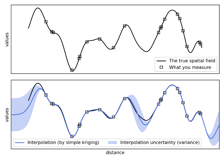
- As a geostatistical method, statistical releationships between locations are calculated and therefore uncertainty estimates are available (unlike in IDW or spline interpolation)
Assumptions
- Assumes that the spatial variation in the phenomenon represented by the z-values is statistically homogeneous throughout the surface (for example, the same pattern of variation can be observed at all locations on the surface)
- Assumes that the distance between sample points reflects a spatial correlation that can be used to explain variation in the surface
Considers not only the distances but also the other variables that have a linear relationship with the estimation variables
Uses a weighted average of the sampled values to predict the value at an unsampled location. The weights are determined by the variogram.
\[\hat Z(s_i) = \sum_{i = 1}^n w_i Z(s_i)\]
- Weights are determined by minimizing the variance of the estimation error, and subject to the constraint that the weights sum to 1.
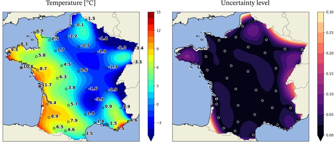
Uses a correlated Gaussian process to guess at values between data points
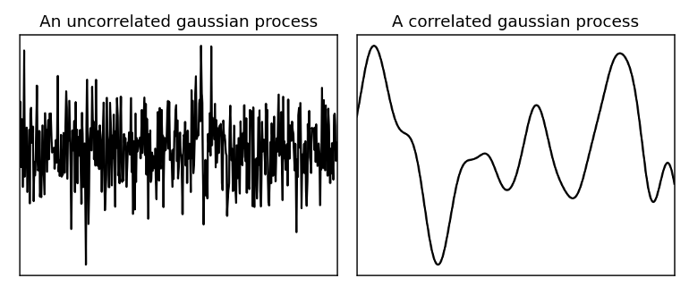
- Uncorrelated - white noise
- Correlated - smooth
- The closer in distance two points are to each other, the more likely they are to have a similar value (i.e. geospatially correlated)
- Example: Temperature
Fewer known points means greater uncertainty
Variograms
Describes the degree of spatial dependence (\(\gamma\)) in a random field or stochastic process (\(Z(s)\) )
- e.g. A measure of how much two samples taken from the mining area will vary in gold percentage depending on the distance between those samples. Samples taken far apart will vary more than samples taken close to each other.
A decrease of spatial autocorrelation is, equivalently, an increase of semivariance
- If your semivariance returns a constant, your data was not spatially related.
Sample (aka Empirical or Experimental) Variogram
\[\begin{align} &\hat \gamma(h_i) = \frac{1}{2N(h_i)} \sum_{j=1}^{N(h_i)} (z(s_j) - z(s_j + h'))^2 \\ &\text{where} \;\; h_i = [h_{i, 0}, h_{i, 1}] \; \text{and} \; h_{i, 0} \le h' \lt h_{i, 1} \end{align}\]
- \(\gamma\) : Spatial dependence between a particular pairwise distance
- \(h\) : Geographical (pairwise) distance between two locations
- \(N(h_i)\) : The number of pairs of locations for that particular distance
- \(z\) : Value of the variable you’re interested in at a particular location. (e.g. Temperature)
- \(s_j\) : Location
The sample variogram cannot be computed at every possible distance, \(h\), and due to variation in the estimation, it is not ensured that it is a valid (?) variogram which is needed for interpolation models. To ensure a valid variogram, models (aka Theoretical Variograms) are used to estimate it.
(Some) Variogram Models
Exponential
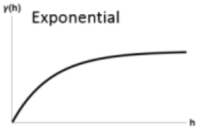
\[\gamma' = p(1- e^{-3h / r}) + n\]
- Spatial autocorrelation (via proxy semi-variance on the Y-Axix) doesn’t completely go to zero until distance (X-Axis) is infinity
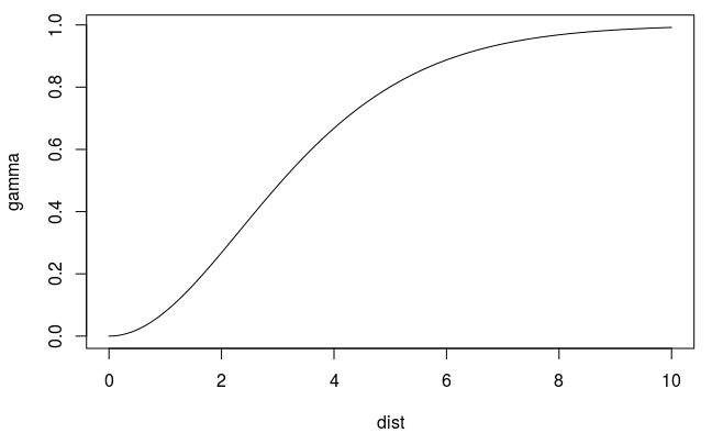
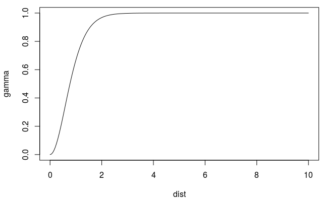
Gaussian
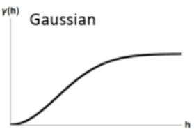
\[\gamma' = p(1 - e^{-(h^2/ (\frac{4}{7}r)^2)}) + n\]
Matern
- Does not allow decreasing or oscillating semivariance (sometimes seen in real data)
- Uses a smoothness parameter, kappa
vgmdefault: 0.5 (which is the Exponential model)- Lower values provide a smoother fit
- Higher values result in a more angular fit
- The Gaussian is when \(\kappa = \infty\)
- fit.kappa = TRUE in
fit.variogramtunes this value- This can be a hindrance to getting a good model and it might be best to tune this on your own.
- For some reason, joint tuning kappa and the model can produce extreme psill and range estimates while resulting in low SSE values
- If you’re getting reasonable estimates with the Exponential model and getting extreme estimates for the Matern (w/fit.kappa = TRUE), I recommend tuning kappa manually on a narrower grid around 0.5. See Geospatial, Spatio-Temporal >> EDA >> Spatial Dependence >> Example 1 >> Block Bootstrapping for a code example
autofitVariogramdefault:c(0.05, seq(0.2, 2, 0.1), 5, 10)
Matern with Stein Parameterization
Spherical
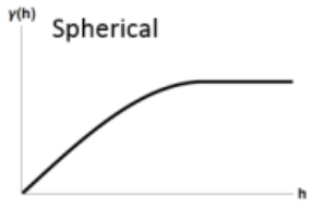
\[\gamma' = \left\{ \begin{array}{lcl} p\left(\frac{3h}{2r} - \frac{h^3}{2r^3}\right) +n & \mbox{if} \; h \le r \\ p + n & \mbox{if} \; h \gt r \end{array}\right.\]
- Spatial autocorrelation goes to zero at some distance
Terms
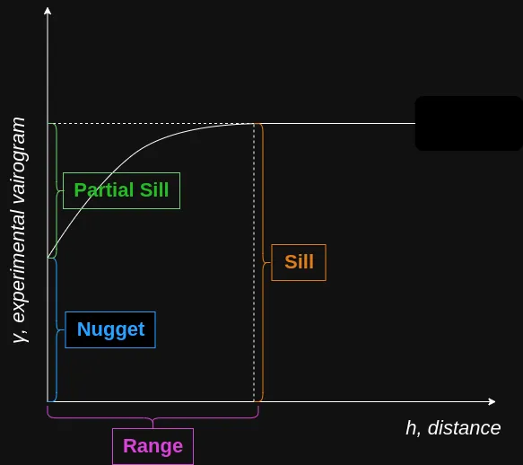
- \(p\): Partial Sill = Sill - Nugget
- The Sill represents the total variance of the variable across the study area.
- \(h\): Pairwise Distance Between Locations
- \(n\): Nugget
- Represents the variability at very small separation distances, often due to measurement errors or micro-scale (smaller than the sampling distances) variations
- Non-negative (i.e. \(\ge 0\))
- A sparse sampling grid can artificially inflate the apparent nugget, because real short-range structure is invisible at that scale
- Nugget-Sill Ratio (Relative Nugget Effect) is the fraction of the total variance is unstructured (random noise or micro-scale variation) versus spatially autocorrelated
Guidelines (Cambardella et al. 1994)
Nugget/Sill Ratio Spatial Dependence < 0.25 (< 25%) Strong — most variance is spatially structured 0.25 – 0.75 (25–75%) Moderate > 0.75 (> 75%) Weak — most variance is noise or micro-scale Consequences
- A low ratio means kriging will perform well, because nearby observations carry strong information about unsampled locations.
- A high ratio means kriging predictions will revert heavily toward the global mean and will not differ much from simple averaging — the spatial structure is too weak to leverage.
- \(r\): Range - The distance in which the difference of the variogram from the sill becomes negligible indictating the pairwise distance at which locations are no longer correlated.
- In models with a fixed sill, it is the distance at which this is first reached
- In models with an asymptotic sill, it is conventionally taken to be the distance when the semivariance first reaches 95% of the sill.
- Positive (i.e. \(\gt 0\))
- \(p\): Partial Sill = Sill - Nugget
Available variogram models in {gstat}
gstat::vgm()
#>     short                                      long
#>  1    Nug                              Nug (nugget)
#>  2    Exp                         Exp (exponential)
#>  3    Sph                           Sph (spherical)
#>  4    Gau                            Gau (gaussian)
#>  5    Exc        Exclass (Exponential class/stable)
#>  6    Mat                              Mat (Matern)
#>  7    Ste Mat (Matern, M. Stein's parameterization)
#>  8    Cir                            Cir (circular)
#>  9    Lin                              Lin (linear)
#>  10   Bes                              Bes (bessel)
#>  11   Pen                      Pen (pentaspherical)
#>  12   Per                            Per (periodic)
#>  13   Wav                                Wav (wave)
#>  14   Hol                                Hol (hole)
#>  15   Log                         Log (logarithmic)
#>  16   Pow                               Pow (power)
#>  17   Spl                              Spl (spline)
#>  18   Leg                            Leg (Legendre)
#>  19   Err                   Err (Measurement error)
#>  20   Int                           Int (Intercept)
Process: Optimize the parameters of variogram model to fit to the sample variogram estimates.
- {gstat} uses weighted least squares to fit the model
- In SDS Ch. 12.3, there’s code to fit an exponential model using maximum likelihood. The range and sill were a little shorter than the WLS fit which made a steeper curve, but they were pretty similar.
- The steeper the curve near the origin, the more influence the closest neighbors will have on the prediction. As a result, the output surface will be less smooth.
- Instead of the constant mean, denoted by
~ 1, a mean function can be specified, e.g. using~ sqrt(dist)as a predictor variable
Preprocessing
- Detrending (trend.beta) - Often improves variogram model regression, but it also removes/diminishes the effects of spatially correlated covariates
- If your semivariance keeps linearly increasing, try de-trending your data.
- I’m not sure how to do this with
variogram’s trend.beta argument. One of the articles uses almin this way:resids_detrend <- lm(resp ~ long + lat, data)$residual- trend.beta asks for the coefficients though.
- Fixing the range can be a performance enhancer for larger data
- Binning method can make a substantial difference on the variogram results
- Types: equal size, equal width, log-spaced binning
- Bins could also be determined by a grouping variable
- If bin size varies, then bins with particularly large or small numbers of observations can produce outlier variogram estimates
- Detrending (trend.beta) - Often improves variogram model regression, but it also removes/diminishes the effects of spatially correlated covariates
Example: Exponential Model
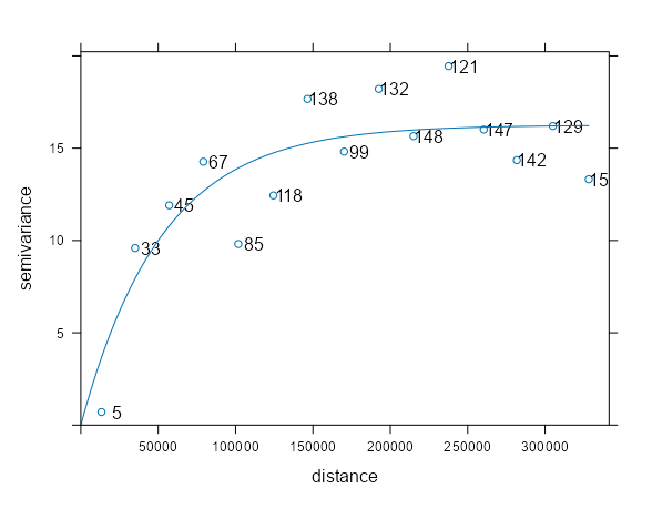
samp_vario <- variogram(NO2 ~ 1, sf_no2) mod_vario <- fit.variogram(samp_vario, vgm(psill = 1, model = "Exp", range = 50000, nugget = 1)) plot(samp_vario, mod_vario, plot.numbers = TRUE)- Data is from IDW Example 1. The fit is pretty decent.
- The points are the sample variogram (
variogram) estimates for the observed locations - The line is the fitted variogram (
fit.variogram) using the sample variogram and the model variogram (vgm) - NO2 ~ 1 specifies an intercept-only (unknown, constant mean) model for (aka ordinary kriging model)
- plot.numbers = TRUE adds the labels which are the number of a location pairs within that pairwise distance interval (pairwise distances are binned here)
- The semivariance is the average of the locations in that bin
- These are the np values from the variogram output
- We see the estimates start to tail downwards past the 300km distance, but the label for that distance bin says that only 15 paired locations went into that sample estimate. So it’s probably noise, and it’d be weird for spatial autocorrelation to suddenly increase at such a large distance.
- Additional
variogramarguments:- cressie: Cressie’s estimator that’s robust against outliers
- cutoff: Maximum spatial separation distance between point pairs that are included in semivariance estimates (Default is one-third of the length of the bounding box diagonal)
- dX: Specifies the delta value of a regressor that determines when location pairs are formed. They are formed only if their regressor vakue difference (euclidean norm) satisfies: \(||x_i - x_j|| \lt \text{dX}\) (i.e. a tolerance/delta value)
- With only one regressor, the euclidean norm is an absolute value of the difference.
- With more than one regressor, this looks like \(\sqrt{(x_{1i} - x_{1j})^2 + (x_{2i} - x_{2j})^2}\) where \(x_1\) and \(x_2\) are regressors (e.g. temperature and wind speed).
- dx = 0.5 and the regressor is a factor says only locations in the same stratum of a “regressor” can be used
- e.g.
PM10 ~ factor(region)) says only distance pairs from the same region - See Geospatial, Spatio-Temporal >> EDA >> Spatial Dependence >> Example 1 for an example where the regressor is a time variable. Therefore, this setting would say that only locations with values (i.e. no NA) in the same time slice (e.g. Apr 14) can form location pairs
- e.g.
- dx = (postive) regressor value says locations that have regressor values with differences up to that value can be paired.
- In pooled temporal variogram example mentioned above, this would say that locations that have values up to and including that difference of time lags can be paired.
- Example: Land Use (rural, urban, forest, etc):
variogram(PM10 ~ land_use, dX = 0.5)- Estimates separate spatial structure within land-use classes (factor variable) without splitting the dataset
- Example: Controlling for a continuous gradient:
variogram(PM10 ~ elevation, dX = 50)- Gives you a spatial variogram of residuals only among stations at similar elevations — e.g. within ±50m — to avoid elevation-driven variance inflating semivariance estimates between lowland and highland stations
- width: The binwidth distance for the location pairs. (Default: cutoff divided by 15)
- There isn’t a need to tune this parameter unless you have few locations and specifically few locations (<100) with short pairwise distances (first few bins of the variogram.
- See Bin Width, Geospatial, Spatio-Temporal >> EDA >> General >> Example: Counts of pairwise distances between locations
- projected = TRUE (default) says you’re using projected coordinates. FALSE is geographic (i.e. decimal degrees).
- Additional
fit.variogramarguments- fit.method: Weighting Options
- Note that these numbers don’t completely correspond to the ones for
- 1: Weights equal to \(N_j\)
- Weights based purely on the number of pairs in the bin
- 2: Weights equal to \(N_j/(\gamma(h_j))^2\)
- Downweights bins based on semivariance
- More adaptive to the shape of your variogram curve than method 7
- 6: Unweighted (OLS)
- 7 (Default): \(N_j/h_j^2\)
- Downweights based on pairwise distance
- Best when you expect a “typically” shaped variogram curve and want to penalize bins of greater pairwise distances
- fit.method: Weighting Options
- The
vgmarguments (besides model) specify starting values in the estimation process. This is not required anymore. It is possible to callvgm("exp")and function will use an algorithm to choose starting values for that model which I think is recommended now.- Also see Geospatial, Spatio-Temporal >> EDA >> Spatial Dependence >> Example >> Block Bootstrapping for a method to get a range of potential starting values (a spatio-temporal case but the code can probably be adjusted for a purely spatial case as well)
- You can compare multiple model types by specifying a vector of model types, e.g.
c("Exp", "Sph"), in which case the best fitting model is returned - Process
- The range parameter is taken as 1/3 of the maximum sample variogram distance,
- The nugget parameter is taken as the mean of the first three sample variogram values, and
- The partial sill is taken as the mean of the last five sample variogram values.
Bin Width
- Also see
- Geospatial, Spatio-Temporal >> EDA >> General >> Example: Counts of pairwise distances between locations
- Bin width matters when the range estimate is unstable due to short-lag bins being too sparse or too noisy.
- Different bin widths push the variogram model optimizer toward different local minima, and kriging predictions can change meaningfully.
- Guidelines
- Use the smallest bin width that gives stable range estimates.
- If stability requires large bins, accept that fine-scale structure (spatial dependence at small distance increments) is unidentifiable.
- Do not tune bin width to “optimize” kriging — that’s chasing noise.
- Approximations assume locations are uniformly distributed across a region and all bins are of equal width.
- Expected Number of Location Pairs (\(N\)) in bin \(k\)
Formula
\[\begin{align} \mathbb{E}[N_k] & = \overbrace{\frac{n(n-1)}{2}}^{\text{total pair count}} \cdot \overbrace{\frac{2h_k\Delta}{H^2}}^{\text{annulus area}}\\ &= \frac{n(n-1)h_k \Delta}{H^2} \end{align}\]
Derivation
- The total location pair count is \(C(n, 2)\)
- The area pf an annulus is \(2\pi h \Delta\), which is like a washer shape, represents a location centered at \(h\) where the inner part of the washer would be the lower bin distance value and the outer part would be the upper. This geometry represents a pair of locations
- The entire area (that we care about) that location pairs are distributed across is a disk of radius \(H\) ( \(\pi H^2\))
- Dividing the annulus by this total are normalizes it (i.e. the integrating of the little \(dh\)s sums equals 1) and gives us a probability distribution which we want for an expected value.
Terms
- \(N_k\) is the number of location pairs in bin \(k\)
- \(n\) is the number of locations
- \(h_k\) is the center distance of the bin interval
- e.g. a bin where h = 10 km and width = 20 has a bin interval of 0 km : 20 km.
- \(\Delta\) is the bin width
- \(H\) is the cutoff
Example: Mid-range bin (center \(\approx\) 100 km)
\[\begin{align} &\mathbb{E}[N] = \frac{53 \cdot 52 \cdot 100 \cdot 20}{200^2} \approx 140 \; \text{location pairs} \\ &\text{where} \;\; n = 53, \;\; h = 100, \;\; \Delta = 20, \;\; H = 200 \end{align}\]
- So if our data has 53 locations, there will likely be around 140 location pairs in the bin centered at a distance of 100 km (with width = 20 and cutoff = 200).
- How many locations for a stable range estimate?
The range estimate is dominated by the first few bins
Formula
\[n \approx \sqrt{\frac{N_k H^2}{h\Delta}}\]
- This is derived by using the expected value formula above. First, by simplifying \(n(n-1)\) to \(n^2\) and then solving for \(n\).
Relative Squared Error for a given number of location pairs
\[\text{RSE} \approx \frac{1}{\sqrt{N_k}}\]
\(N_k\) RSE 25 ~20% 50 ~14% 100 ~10% 200 ~7% - 10% or less can be probably be considered a pretty stable estimate
Example: First Bin (center \(\approx\) 10 km)
\[\begin{align} &n \approx \sqrt{\frac{100\cdot 200^2}{10 \cdot 20}} = 140\\ &\text{where} \;\; m = 100, \; H = 200, \; h = 10, \; \Delta = 20 \end{align}\]
- \(N_k\) is the desired number of location pairs in bin \(k\)
- So to get a solid estimate of the range, we’d need around 140 locations under the assumptions that they are uniformly distributed and we’re using equal width bins.
- What should my bin width be?
The context is that we want a good range estimate, so a low error rate in the first few bins is desired. The other side is that we also need enough total bins for a curve (variogram model) estimate, so we can’t make the width too large.
Therefore, we want the minimum bin size so that the first bin has a low enough error rate but doesn’t affect the curve fit.
Ideally:
- At least 100 location pairs in the first bin
- There should 6–8 bins before the sill (to fit the variogram model)
If you have close to the ideal location pair count in the first bin, then the default bin width (cutoff / 15) is probably fine. Otherwise, try workflow below.
Workflow
Choose \(N_{\text{min}}\) (See RSE table) (e.g. 75 effective pairs)
Compute \(\Delta_{\text{min}}\)
\[\Delta_{\text{min}} = \sqrt{\frac{2N_{\text{min}}H^2}{n(n-1)}}\]
Assess sensitivity of range estimate for \(\Delta \gt \Delta_{\text{min}}\) (Code in Geospatial, Spatio-Temporal >> EDA >> Spatial Dependence >> Example >> Block Bootstrapping can be probably be adjusted to do this)
- Fit models
- If, for example, \(\Delta_{\text{min}} \approx 40\) , then start with \(\Delta = 40\) which is width = 40
- For example, with 53 locations, the first bin at this width would have ~60 pairs; noisy but usable.
- Fit only simple variogram models (Exp, spherical) with and without nugget
- Optionally, drop the first bin (
vario_samp[-1, ]) of the empirical variogram and fit the model. A large change in the range estimate could indicate non-spatial microscale effects (See Geospatial, Spatio-Temporal >> Terms) are present.
- Optionally, drop the first bin (
- Collect range estimates
- If, for example, \(\Delta_{\text{min}} \approx 40\) , then start with \(\Delta = 40\) which is width = 40
- Repeat for \(\Delta = 30, 20, 15, \text{and maybe}\;50\)
- Fit models
Interpret results
Sensitivity outcome What you observe Interpretation Implication for final model Range stable across Δ ≥ Δ_min, no nugget Similar range for multiple bin widths Spatial correlation exists at that scale conditional on smoothness Use Δ_min Range unstable for Δ ≈ Δ_min but stabilizes for larger Δ Range varies wildly at small bins, settles as Δ increases Short-lag bins too noisy; geometry limits resolution Use larger Δ in final model Range stable w.r.t. Δ but shifts substantially when nugget added Nugget absorbs short-lag variance; range increases Intrinsic microscale effects are possible Report range with nugget and qualify interpretation Range unstable w.r.t. both Δ and nugget No consistent range under any specification Spatial dependence weak or absent Avoid spatial model; or use strong regularization Removing first bin has little effect Range essentially unchanged Any instability is structural, not outlier-driven Use all bins; focus on model assumptions Removing first bin changes range materially Large shift in range Intrinsic microscale effects are possible Either increase Δ or include nugget Nugget ≈ large fraction of sill Nugget comparable to psill Most variability non-spatial at observed scale Expect weak performance using kriging Nugget ≈ 0 with stable range Nugget not selected by optimizer Strong spatial continuity Spatial prediction likely effective - First row: “Conditional on smoothness” refers to there being a continuous relationship between distance and semi-variance.
- Third row: Says that if the model estimates a nugget when given the opportunity, then there might not be enough locations or that there could be some non-spatial microscale effects at work.
- Any reporting of the range estimate (with nugget) should state that the model was not able to resolve spatial dependence below the first bin distance.
- Sixth row: In terms of nonspatial microscale effects, the first bin is the most likely one to be contaminated. If the first bin is dominating the fit, then some extra investigation should be done at that scale.
Types
Simple Kriging (SK) - Assumes the mean of the process is known and constant across the entire domain — you have to specify it explicitly. It’s rarely used in practice because you almost never know the true mean. (e.g.
pm10 ~ 0)Ordinary Kriging (OK) - Assumes that the mean of the study variable is the same everywhere and spatial variability is a random process. (e.g.
pm10 ~ 1). This is the most commonly used form of kriging.- The
~ 1in the formula means “estimate a constant mean from the data.” - The kriging system includes an unbiasedness constraint that implicitly estimates this unknown mean as part of the prediction.
- The
Universal Kriging (UK) (aka Regression-Kriging (RK), ) - Assumes that there is an overriding trend in the data — the mean varies across the domain as a function of covariates. (e.g.
pm10 ~ wind_speed)
\[\begin{align} \hat z (s_0) &= \hat m(s_0) + \hat e(s_o)\\ &= \sum_{k=0}^p \hat \beta_k q_k(s_0) + \sum_{i=1}^n \lambda_i e(s_i) \end{align}\]
- Terms
- \(\hat m (s_0)\) : Fitted deterministic part at location, \(s_0\)
- \(\hat e (s_0)\) : Interpolated residual
- \(\lambda_i\) : Kriging weights determined by variogram
- \(q\) : Covariates
- Includes other variables that are meaningfully correlated with the target variable in the kriging model to account for trend
- In ordinary Kriging and conditional simulation (without covariates), it’s assumed that all spatial variability is a random process, characterized by a spatial covariance model.
- Adding variables typically reduces both the spatial correlation in the residuals, as well as their variance, and leads to more accurate predictions and more similar conditional simulations.
- Process: The regression-part is estimated. Then, the residual is interpolated with kriging and added to the estimated trend.
- Some authors reserve the term universal kriging (UK) for the case when only the coordinates are used as predictors. If the deterministic part of variation (drift) is defined externally as a linear function of some auxiliary variables, rather than the coordinates, the term kriging with external drift (KED) is preferred
- Terms
Block Kriging - Uses all the data (i.e. data weighted by distance) to estimate the mean of the variable over the target areas (i.e. polygons)
- It smooths the mean estimate of the area by using the values from neighbors, and by using more data, the estimate has smaller standard errors than just calculating sample means independently.
- Using
aggregategets you the sample mean per area. Block kriging doesn’t assume the average value estimate is independent of neighboring areas.
Conditional Simulation
- Uses the data of the convenience sample as conditioning data and applies Monte Carlo simulation which results in a distribution of a statistic.
- See
- SSWR, Ch.13.1.2 for an example of unconditional simulation where locations are (regularly) randomly sampled and the variance of overall mean (population) estimates is calculated. External variables are included in the variogram and kriging models to account for “trend.”
- (SDS, Ch.12.6) for a basic example of conditional simulation
- Conditional simulation is only recommended if the quality of the data is sufficient, and we may trust that the study variable at the points has not changed since these data have been collected.
- Otherwise Unconditional Simulation (aka Indicator Simulation) is recommended.
krige(nsim = 1, indicator = TRUE)where indicator = TRUE enforces unconditional simulation
- Otherwise Unconditional Simulation (aka Indicator Simulation) is recommended.
- Conditional Simulation Process (SDS, Ch.12.6)
- Carry out a kriging prediction
- Draw a random variable from the normal distribution with mean and variance equal to the kriging variance
- Adds this value to the conditioning dataset
- Find a new random simulation location and repeat process
- Unconditional Simulation Process (SSWR, Ch.13.1.2)
- Select a large number S of random samples with sampling design p.
- Use the model to simulate values of the study variable for all sampling points.
- Estimate for each sample the population mean, using the design-based estimator of the population mean for sampling design p. This results in S estimated population means.
- Compute the variance of the S estimated means.
- Repeat steps 1 to 4 R times, and compute the mean of the R variances.
- For larger datasets, use
krigeSimCE(circular embedding method) orkrigeSTSimTB(turning bands method)
Examples
Example 1: Ordinary Kriging of NO2 in Germany
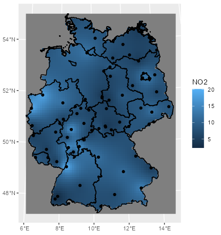
mod_krig_no2 <- krige(formula = NO2 ~ 1, locations = sf_no2, newdata = grid_de, model = mod_vario) ggplot() + # interpolation fill geom_stars(data = mod_krig_no2, aes(x = x, y = y, fill = var1.pred)) + labs(fill = "NO2") + xlab(NULL) + ylab(NULL) + # polygons to multistring geom_sf(data = st_cast(shp_de, "MULTILINESTRING")) + # points geom_sf(data = sf_no2) + coord_sf(lims_method = "geometry_bbox")- NO2 ~ 1 specifies an intercept-only (unknown, constant mean) model for (aka ordinary kriging model)
- sf_no2 contains observed location geometries (See Inverse Distance Weighting (IDW) >> Example 1)
- grid_de is a grid for predicting values at new locations (See Inverse Distance Weighting (IDW) >> Example 1)
- mod_vario is the fitted variogram model (See Variograms >> Example 1)
Example 2: Block Kriging NO2 in Germany
pacman::p_load( dplyr, ggplot2, sf, gstat ) df_no2_agg <- aggregate(sf_no2["NO2"], by = shp_de, FUN = mean) df_krig_no2 <- krige(NO2 ~ 1, locations = sf_no2, newdata = shp_de, model = mod_vario) tib_krig_samp <- df_krig_no2 |> mutate(sample_mean = df_no2_agg$NO2) |> select(krig_mean = var1.pred, sample_mean) |> # go longer and coerce to factor for facet_wrap tidyr::pivot_longer( cols = 1:2, names_to = "agg_type", values_to = "no2_mean" ) |> # change categories/levels for nicer facet titles mutate(agg_type = forcats::fct_recode(agg_type, Kriging = "krig_mean", Sample = "sample_mean")) head(tib_krig_samp) #> Simple feature collection with 6 features and 2 fields #> Geometry type: MULTIPOLYGON #> Dimension: XY #> Bounding box: xmin: 388243.2 ymin: 5235822 xmax: 855494.6 ymax: 5845553 #> Projected CRS: WGS 84 / UTM zone 32N #> # A tibble: 6 × 3 #> geometry agg_type no2_mean #> <MULTIPOLYGON [m]> <fct> <dbl> #> 1 (((546832.3 5513967, 546879.7 5512723, 547306.1 5512316, 546132.9 5511048, 546977.6 ... Kriging 9.02 #> 2 (((546832.3 5513967, 546879.7 5512723, 547306.1 5512316, 546132.9 5511048, 546977.6 ... Sample 8.14 #> 3 (((580328.6 5600399, 580762.2 5599574, 581595.4 5599590, 581578.3 5600424, 582410.7 ... Kriging 9.04 #> 4 (((580328.6 5600399, 580762.2 5599574, 581595.4 5599590, 581578.3 5600424, 582410.7 ... Sample 10.0 #> 5 (((802977.3 5845553, 803005.9 5844726, 803829.3 5844758, 803844.2 5844345, 803460.6 ... Kriging 12.0 #> 6 (((802977.3 5845553, 803005.9 5844726, 803829.3 5844758, 803844.2 5844345, 803460.6 ... Sample 12.2- To go from kriging to block kriging, we replace the grid (grid_de) with polygons (shp_de) in newdata
- sf_no2 contains observed location geometries (See Inverse Distance Weighting (IDW) >> Example 1)
- shp_de is the shapfile object with the polygons (See Inverse Distance Weighting (IDW) >> Example 1)
- mod_vario is the fitted variogram model (See Variograms >> Example 1)
calc_samp_se <- function(x) sqrt(var(x)/length(x))
df_samp_se <-
  aggregate(sf_no2["NO2"],
            shp_de,
            calc_samp_se)

tib_krig_samp_se <-
  df_krig_no2 |>
  mutate(sample_mean_se = df_samp_se$NO2,
         krig_mean_se = sqrt(var1.var)) |>
  select(krig_mean_se, sample_mean_se) |>
  tidyr::pivot_longer(
    cols = 1:2,
    names_to = "agg_type",
    values_to = "no2_mean_se"
  ) |>
  mutate(agg_type = forcats::fct_recode(agg_type,
                                        Kriging = "krig_mean_se",
                                        Sample = "sample_mean_se"))
Block Kriging Means vs Sample Means
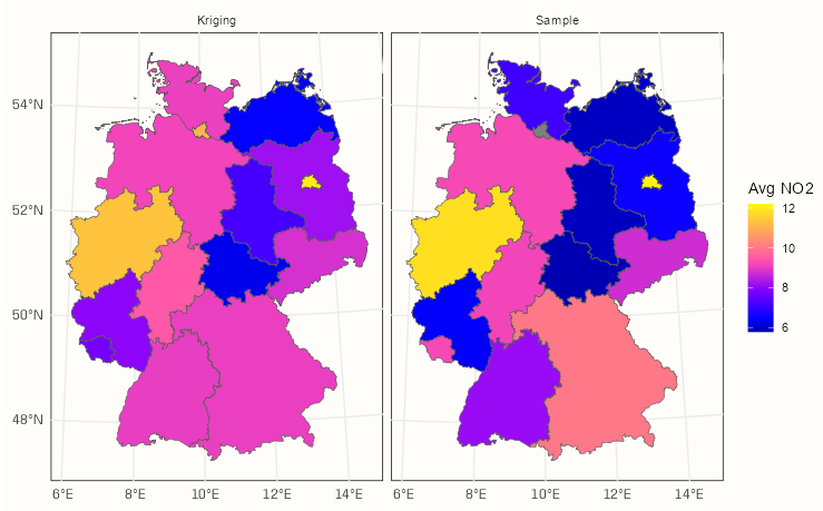
ggplot() + geom_sf(data = tib_krig_samp, mapping = aes(fill = no2_mean)) + facet_wrap(~ agg_type) + scale_fill_gradientn(colors = sf.colors(20)) + labs(fill = "Avg NO2") + theme_notebook()- With the block kriging, the mean of an area gets smoothed towards it’s neighborhood mean. This typically results in the more higher sample means being lessened and the more lower sample means being increased
Block Kriging SEs vs Sample SEs
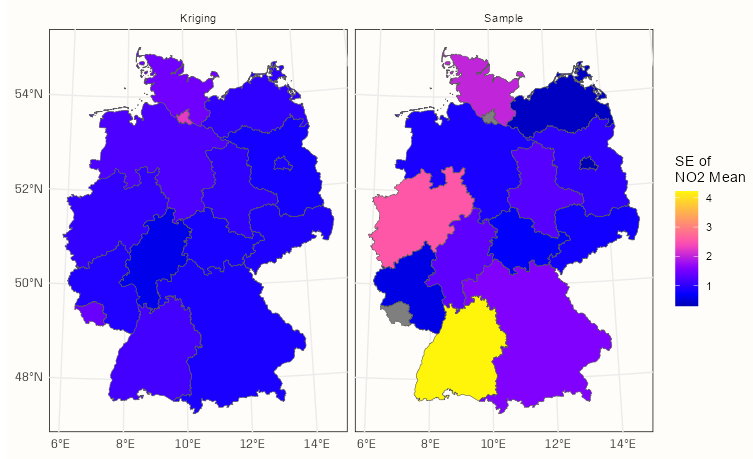
ggplot() + geom_sf(data = tib_krig_samp_se, mapping = aes(fill = no2_mean_se)) + facet_wrap(~ agg_type) + scale_fill_gradientn(colors = sf.colors(20)) + labs(fill = "SE of \nNO2 Mean") + theme_notebook()- By including all the data in the means calculations, kriging achieves substantially smaller standard errors than many of those calculated for the sample means.
Example 3: Universal Kriging
- German population density is used as a predictor for NO2 concentration in air.
- Population data is from a recent census
- The population data used to calculate the population density variable needed to be aggregated from a 100m grid cell to the 10km grid cell of the NO2 response variable.
- For code, see Geospatial, Preprocessing >> Aggregations >> Examples >> Example 5
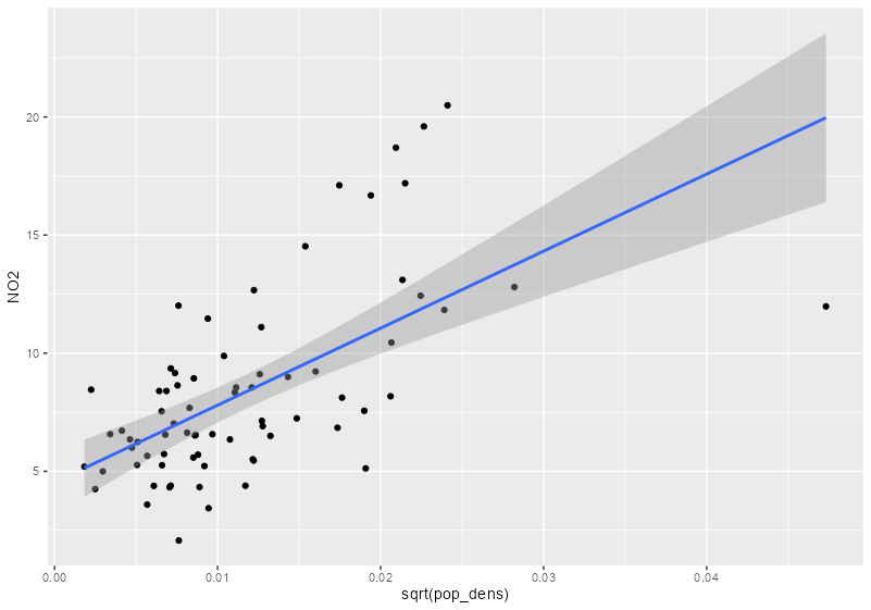
sf_no2_popdens <- grid_de |> select(pop_dens) |> st_extract(sf_no2) |> mutate(pop_dens = as.numeric(pop_dens)) |> filter(!is.na(pop_dens)) |> st_drop_geometry() |> # redundant geometry bind_cols(sf_no2) |> # strips sf class st_as_sf() # adds sf class back # no2 vs pop dens ggplot(sf_no2_popdens, aes(x = sqrt(pop_dens), y = NO2)) + geom_point() + geom_smooth(formula = "y ~ x", method = "lm")- grid_de is a stars object which is a list with attributes.
st_extractcombines the values from the stars object to the locations specified by a sf object and returns a sf dataframe.
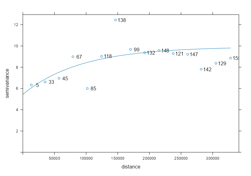
# sample variogram var_samp_no2 <- variogram(NO2 ~ sqrt(pop_dens), sf_no2_popdens) # model variogram var_mod_no2 <- fit.variogram(var_samp_no2, vgm(1, "Exp", 50000, 1)) plot(x = var_samp_no2, model = var_mod_no2, plot.numbers = TRUE)- Outliers at 100K and 150K meters, but otherwise the fit seems decent
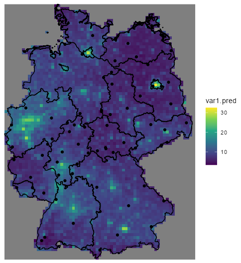
no2_krig_univ <- krige(formula = NO2 ~ sqrt(pop_dens), locations = sf_no2_popdens, newdata = grid_de["pop_dens"], model = var_mod_no2) ggplot() + geom_stars(data = no2_krig_univ, aes(x = x, y = y, fill = var1.pred)) + geom_sf(data = st_cast(shp_de, "MULTILINESTRING")) + geom_sf(data = sf_no2) + scale_fill_viridis_c() + coord_sf(lims_method = "geometry_bbox") + theme_void()- Only rural locations were selected, so the data is geographically biased. The model doesn’t having any information about NO2 concentrations in high population density areas, so the NO2 predictions for urban centers follow closely with population density estmates.
- i.e. the higher the population density, the higher the predicted concentration of NO2.
- Therefore, predictions for high population density areas shouldn’t be considered reliable.
- Also, apparently pollution in rural and urban have different “processes” (circulation?, monitoring?) and should be modelled separately. ({gstat} vignette, section 3)
- German population density is used as a predictor for NO2 concentration in air.