Sampling Methods
Misc
- Also see Surveys, Analysis >> Weights >> Types >> Replicate Weights
- A way of not disclosing your sampling method for security/privacy reasons
- Notes from:
- Survey data in the field of economy and finance (ebook)
- Ch. 10 Sample Designs and Replicate Weights ({srvyr} book)
- Packages
- {samplex} - An interactive ‘shiny’ application to assist in determining sample sizes for common survey designs such as ‘simple random sampling’, ‘stratified sampling’, and ‘cluster sampling’.
- {SampleSelectR} - Supports the design and implementation of common survey sampling methods. It is designed to make sample design and selection reproducible, efficient, and transparent for survey statisticians and researchers.
- {samplyr} - A tidy grammar for survey sampling in R.
- Provides a minimal set of composable verbs for stratified, clustered, multi-stage, and multi-phase sampling designs with PPS methods, sample coordination, and panel rotation.
- {SscSrs} - Sample Size Calculator for Estimation of Population Mean and Proportion under SRS
- Resources
Terms
- In a survey setting,
- U - Denotes a finite population (i.e. [target population) of N units
- A sample s of n units (n≤N) is taken from U
- Design Weights - The average number of units in the population that each sampled unit represents. This weight is determined by the sampling method and is an important part of the estimation process.
- Estimator of the parameter, \(\theta\), is a function of sample observations
Example: Sample Mean
\[ \hat{\theta} = \frac {\sum_{i \in S}y_i}{S} = \bar{y}_S \]
- Population mean of the study variable can be estimated by the mean value over the sample observations
- Inclusion Probability - The probability for a unit to appear in the sample
- Study Parameter (\(\theta\)) - Linear parameter of the study variable, such as a mean, a total or a proportion, or a more complex one such as a ratio between two population means, a correlation or a regression coefficient, a quantile (e.g. median, quartile, quintile or decile) or an inequality measure such as the Gini or the Theil coefficient. (also see estimator)
- Study Variable (\(y\))
- Quantitative - Numerical information (e.g. the total disposable income or the total food consumption)
- Qualitative - Categorical information (e.g. gender, citizenship, country of birth, marital status, occupation or activity status)
Probabilistic Sampling Methods
Simple Random Sampling (SRS)
A method of selecting n units out of N such that every sample s of size n has the same probability of selection
Simple Inclusion Probability - the probability for a unit to appear in the sample
\[ \pi_i = \mbox{Pr}(i \in S) = \sum \limits_{i \in s \in S} \mbox{Pr}(S = s) = \frac {\binom{N-1}{n-1}}{\binom{N}{n}} = \frac {n}{N} \]
- \(n\) is the size of sample, \(s\), and \(N\) is the target population size
Double Inclusion Probability - the probability for 2 units to appear in the sample
\[ \pi_{ij} = \mbox{Pr}(i,j \in S) = \sum \limits_{i,j \in s \in S} \mbox{Pr}(S = s) = \frac {\binom{N-2}{n-2}}{\binom{N}{n}} = \frac {n}{N} \frac {n-1}{N-1} \]
- Where \(i \neq j\)
- \(n\) is the size of sample, \(s\), and \(N\) is the target population size
Without Replacement (most common)
- At the first extraction, each one of the population units will have an equal probability of selection, \(1/N\).
- At the second extraction, the remaining N-1 units will have a selection probability equal to \(1/(N-1)\). Etc.
With Replacement - all the units of the population will have all the same probability of being selected \(1/N\) Advantages:
- It’s simple and doesn’t use auxiliary information on the population
- The selection is random and, then, any unit is favoured
- The sample is representative Disadvantages:
- The choice of the element is completely random
- A complete list of the population units is necessary
- It’s time and cost consuming
Estimated Total of the study variable, \(\hat{Y}\)
\[ \hat{Y}_{SRS} = N \bar{y} \]
- Where \(N\) is the target population size
Estimated Mean of the study variable, \(\bar{Y}\)
\[ \hat{\bar{Y}}_{SRS} = \bar{y} \]
- Where \(\bar{y}\) is the sample mean
Variance for Estimated Total
\[ V(\hat{Y}_{SRS}) = N^2 (1-f) \frac {S^2_y}{n} \]
\(S^2_y\) is the dispersion of the study variable, \(y\), over the population \(U\)
\[ S^2_y = \frac {1}{N-1} \sum_{i \in U} (y_i - \bar{Y})^2 \]
Sampling Rate or Sampling Fraction: \(\mbox{f} = n/N\)
Finite Population Correction Factor: \(1-\mbox{f}\)
Variance for Estimated Mean
\[ \hat{V}(\bar{y}) = (1-\mbox{f}) \frac {s^2_y}{n} \]
Sample Dispersion
\[ s^2_y = \frac{1}{n-1}\sum_{i \in s} (y_i - \bar{y})^2 \]
Estimated size of subpopulation, \(A\)
\[ \hat{N}_A = Np_A \]
- \(p_A\) is the sample proportion of units from target subpopulation, \(U_A\)
- i.e. (I think) \(n_A / N_A\)
- Examples: Subpopulations
- Total number of males or females in the population
- Total number of elderly people aged more than 65 in the population
- Total number of establishments having more than 50 employees in a certain geographical region or in a sector of activity.
- \(p_A\) is the sample proportion of units from target subpopulation, \(U_A\)
Variance of sample proportion of subpopulation, \(A\)
\[ \hat{V}(p_A) = \frac{p_A(1-p_A)}{n} \]
Domain Parameter Estimation
Refers to estimating population parameters for sub-populations of interest, called domains. For instance, one may wish to estimate the mean household disposable income broken down by personal characteristics such as age, gender or citizenship
- I think this is different from “Estimated size of subpopulation, A” (above) because we’re estimating a study variable of subpopulation vs the size of the subpopulation
Estimated Total of the study variable
\[ \hat{Y}_D = \frac{N \cdot n_D}{n} \; \bar{y}_D \]
\(\bar{y}_D\) - The sample mean of study variable, \(y\), within the domain, \(D\)
\(n_D\) - The total number of sample units from the sample \(s\) which fall into domain, \(D\)
- Sample size \(n_D\) is a random variable of mean \(\bar{n}D = nP_D\) where \(P_D = N_D / N\)
- I guess this is a random variable because this is strictly SRS, so you aren’t stratifying by \(D\) when you sample the target population. Therefore, the number of samples from \(D\) you happen to get will be random and have a distribution.
- Sample size \(n_D\) is a random variable of mean \(\bar{n}D = nP_D\) where \(P_D = N_D / N\)
Alternative: When the size of the domain, \(N_D\), of \(U_D\) is known
- \(\hat{Y}_{D,\mbox{alt}} = N_D \cdot \bar{y}D\)
- This formula has a provably (see ebook in Misc) lower variance than the original formula
Variance for Estimated Total
\[ V(\hat{Y}_D) \approx N^2_D \left(\frac{1}{\bar{n}_D} - \frac{1}{N_D}\right)S^2_D \left(1 + \frac{1-P_D}{CV^2_D} \right) \]
Where
\[ \begin{align} &S^2_D = \sum_{k \in U_D} \frac{(y_k - \bar{Y}_D)^2}{N_D - 1}\\ &CV_D = \frac{S_D}{\bar{Y}_D} \end{align} \]
Assumes the population sizes, \(N\) and \(N_D\), are “large enough.”
For the Alternative Estimated Total formula (see above)
\[ V(\hat{Y}_{D,alt}) \approx N^2_D \left(\frac{1}{\bar{n}_D} - \frac{1}{N_D} \right)S^2_D \]
- Assumes the sample size, \(n_D\), is “large enough.”
- A provably lower variance (see ebook in Misc)
Unequal Probability Sampling
Different units in the population will have different probabilities of being included in a sample.
- Unlike SRS, where each unit has an equal probability of being included in the sample
Unequal probability sampling can result in estimators having higher precision than when simple random sampling or other equal probability designs are used.
- Emphasizes the importance of utilizing so-called “auxiliary” information as a way to boost sampling precision. (see πk below)
Often the probability of selection is chosen to be proportional to some measure of size, such as in sampling with Probabilities Proportional to Size (PPS)), particularly when sampling Primary Sampling Units (PSU) in a multi-stage or multi-phase sample. Units with larger size measures are more likely to be sampled
- A size measure is constructed for each unit (e.g., the population of the PSU or the number of occupied housing units)
Systematic Sampling is commonly used to ensure representation across a population. Units are sorted by a feature, and then every \(k\) units is selected from a random start point so the sample is spread across the population.
Example: Establishment Survey
- A company wants to determine a “manufacturer’s suggested retail price” or “MSRP”. So, they survey all the stores (i.e. establishments) that sell their product.
- Along with the usual components of the frame, it lists the volume of sales of the product and sale price.
- The probability of selection for each establishment is proportional to its sales volume of the products. (i.e. probabilities proportional to size or PPS)
- A sample is taken using that PPS and a simple average of prices from those selected establishments will be an unbiased estimate of the average price of units sold.
Horvitz-Thompson estimator (without replacement selection)
Estimated Total, \(\hat{Y}\), for the study variable
\[ \hat{Y}_{HT}= \sum_{k \in S} \frac{y_k}{\pi_k} = \sum_{k \in s} d_ky_k \]
\(d_k = 1/\pi_k\) is the design weight of unit, \(k\), of sample, \(s\)
\(\pi_k\) is the inclusion probability for unit, \(k\), of sample, \(s\)
- In practice, as the study variable \(y\) is unknown, the inclusion probabilities should be taken proportional to an auxiliary variable \(x\) assumed to have a linear relationship with \(y: π \propto x\) (probability proportional to size sampling)
- An inclusion probability that is optimal with respect to one study variable may be far from optimal with other study variables. In case of multi-purpose surveys, this is a major problem which generally prevents from using unequal probability sampling.
- Alternatively, survey statisticians use stratification as we know it always make accuracy better no matter the study variable.
Hansen-Hurwitz estimator has been proposed in case of sampling with replacement.
Cluster Sampling
- Also see Unequal Probability Sampling which is often combined with Cluster designs
- Assumes population has natural clusters (e.g. family unit). Different from Stratified Sampling in that the clustering characteristic(s) is the same for all clusters (between cluster variation = 0) and the within cluster variation is heterogeneous (i.e. within cluster variation != 0).
- Often used when a list of the entire population is not available or data collection involves interviewers needing direct contact with respondents.
- Clusters are commonly structural, such as institutions (e.g., schools, prisons) or geography (e.g., states, counties).
- Example: Family units in NYC are chosen randomly chosen. The variation between family members is whats studied.
- Clusters can also be called Primary Sampling Units (PSU).
- The simplest design involves sampling clusters and then sampling the units within the clusters. In more complex designs, the cluster/sampling process can occur for multipl levels.
- Advantages:
- it’s efficient when the clusters constitute naturally formed subgroups, for which we don’t possess the list of the population
- Studying clusters can be less expensive than simple random sampling.
- Interviewers are sent to specific sampled areas rather than completely at random across a country
- Disadvantages:
- The conditions of the clusters aren’t always respected. The clusters may contain similar elements.
- Compared to a simple random sample for the same sample size, clustered samples generally have larger standard errors of estimates.
- Example
- Students in which a given number of schools are selected, and then students are sampled within each of those chosen schools or clusters.
- In this case, the schools are called the ‘‘primary sampling units’’ (PSUs), while the students within the schools are referred to as the ‘‘secondary sampling units’’ (SSUs).
Stratified Sampling
Misc
- Notes from Chapter 3 Stratification
- Resources
- Cube Method (Haven’t read yet, but looks interesting)
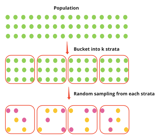
- The population is classified into subpopulations, called strata, based on some categorical characteristics, such as age, gender, education
- Stratified sampling buckets the population into k strata (e.g., countries), and then the experiment random samples individuals from each stratum independently.
- Assumes between group variation is not 0 (i.e. heterogeneous) and within-group variation is 0 (i.e. homogeneous)
- Reasons for stratification
- Baseline for group A different from group B
- Reason to believe the effect for group A will be different from group B
- Advantages
- If the strata are correlated with survey outcomes, a stratified sample has smaller standard errors compared to a SRS sample of the same size.
- There is less risk of obtaining non-representative samples
- Disadvantages
- It needs the availability of auxiliary information on the population.
- There are strict conditions for the strata
- Examples
- A population of North Carolina residents could be stratified into urban and rural areas, and then an SRS of residents from both rural and urban areas is selected independently. This ensures there are residents from both areas in the sample.
- Law enforcement agencies could be stratified into the three primary general-purpose categories in the U.S.: local police, sheriff’s departments, and state police. An SRS of agencies from each of the three types is then selected independently to ensure all three types of agencies are represented.
- Ranked Set Sampling
- Notes from
- Packages
- {generalRSS} (Paper) - Provides extensive tools for both BRSS and URSS, addressing limitations in existing RSS software that primarily focus on balanced designs.
- Supports RSS data generation, efficient sample allocation strategies for URSS, and statistical inference for both balanced and unbalanced designs
- Paper has two medical data applications: a one-sample mean inference and a two-sample area under the curve (AUC) comparison
- {generalRSS} (Paper) - Provides extensive tools for both BRSS and URSS, addressing limitations in existing RSS software that primarily focus on balanced designs.
- Utilizes auxiliary information for ranking and stratification
- Balanced RSS (BRSS) assumes equal allocation across strata
- Unbalanced RSS (URSS) allows unequal allocation, making it particularly effective for skewed distributions.
- Process
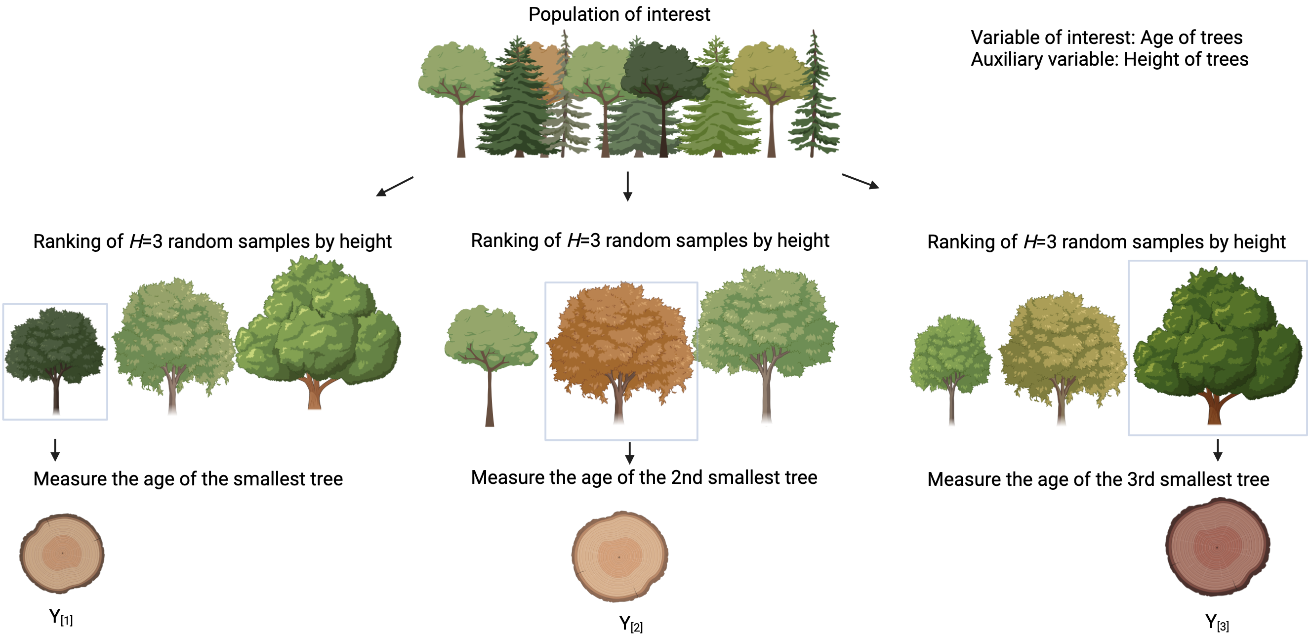
- Select a simple random sample of size \(H\) from the target population
- Rank the \(H\) sampled units using an auxiliary variable without measuring the variable of primary interest.
- Measure the unit ranked as the h-th smallest and discard the remaining units
- Repeat Steps 1-3 for each rank \(h\) up to \(H\).
Estimated Total, \(\hat{Y}\), for the study variable and the
Estimated Mean of the study variable, \(\bar{Y}\) (respectively)\[ \begin{align} &\hat{Y}_\mbox{STSRS}=\sum_{h=1}^H N_h \bar{y}_h \\ &\hat{\bar{Y}}_\mbox{STSRS} = \sum_{h=1}^H W_h \bar{y}_h \end{align} \]
- Assumes SRS within each strata
- \(N\) is the population size
- \(N_h\) is the population strata size for strata, \(h\)
- \(W_h\) is the frequency weight where \(W_h = N_h / N\)
- \(\bar{y}_h\) is the sample mean of strata, \(h\)
Variance for Estimated Total (assuming SRS within strata)
\[ V(\hat{Y}_\mbox{STSRS}) = \sum_{h=1}^H N_h^2 (1-\mbox{f}_h)\frac{S_h^2}{n_h} \]
- \(n_h\) is the sample size for stratum, \(h\)
- Stratum Sampling Fraction: \(\mbox{f}_h = n_h / N_h = n/N\) (which is just \(\mbox{f}\))
- Assumes \(\mbox{f}_h\) is the same for each strata
- Stratum Dispersion: \(S_h^2\) should be similar to the sample dispersion for SRS below, except the domain of the variables is within stratum, \(h\) (e.g. \(n → n_h,\) \(ȳ → ȳ_h\), etc.)
Sample Dispersion for SRS
\[ s_y^2 = \frac{1}{n-1}\sum_{i \in s} (y_i - \bar{y})^2 \]
Variance for Estimated Mean (assuming SRS within strata)
\[ V(\bar{Y}_\mbox{STSRS}) = (1 - \mbox{f}) \frac{s^2_h}{n_h} \]
\(n_h\) will be the same for all \(h\), so it’s constant in this case
Sampling Fraction: \(\mbox{f} = N / n\)
- \(n\) is the overall sample size
Within-Stratum Dispersion
\[ S_w^2 = \sum_{h=1}^H W_hS_h^2 \]
- \(S^2_h\): See above
- \(N\) is the population size and \(N_h\) is the population strata size for strata, \(h\)
- \(W_h\) is the frequency weight where \(W_h = N_h / N\)
Design Weights: \(d_i = N_h / n_h \;\;\forall \in s_h\)
- For SRS, design weights are equal within each stratum
- \(s_h\) is the set of samples within stratum, \(h\)
Stratum sample size allocation methods
Let assume the overall sample size, \(n\), has been fixed (generally out of budgetary considerations). We seek to determine which sample size, \(n_h\), is to be drawn out of each stratum in order to achieve statistical optimality under cost considerations.
When strata are explicit, algorithms such as Neyman allocations for single estimands or the Chromy allocation algorithm for multiple estimands may be used to decide how many units to select from each stratum.
Equal Allocation
- \(n^\mbox{eq}_h = n / H\)
- \(H\) is the number of strata
- Performs poorly when the dispersions, \(S^2_h\), are different from one stratum to another
Proportional Allocation
Consists of selecting samples in each stratum in proportion to the size, \(N_h\), of the stratum population
\(n^\mbox{prop}_h = (n \cdot N_h) / N = n \cdot W_h\)
Variance
\[ \begin{align} V(\hat{\bar{Y}}_\mbox{prop}) &= (1-\mbox{f})\frac{S^2_w}{n} \\ &=\frac{\sum_{h=1}^h W_h S^2_h}{n} - \frac{\sum_{h=1}^h W_h S^2_h}{N} \end{align} \]
Optimal or Neyman Allocation
Seeks to minimize the variance under the cost constraint
\[ \sum_{h=1}^H c_h n_h = C_0 \]
- \(C_0\) is the overall budget available and \(c_h\) the average survey cost for an individual in stratum \(h\).
Strata Sample Size with Cost Constraint
\[ \forall h \;\; n_h^\mbox{opt} = \frac{N_hS_h}{\sqrt{c_h}} \frac{C_0}{\sum_{h=1}^H N_h S_h \sqrt{c_h}} \]
Strata Sample Size without Cost Constraint
\[ n_h^\mbox{opt} = n \frac{N_hS_h}{\sum_{h=1}^H N_hS_h} \]
Variance
\[ V(\hat{\bar{Y}}_\mbox{SRS}) = \frac{1}{n}\sum_h W_h(\bar{Y}_h - \bar{Y})^2 - \frac{1}{n}\sum_h W_h(S_h - \bar{S})^2 \]
- \(\bar{S}\) must be the mean sqrt dispersion across all stratum
Contrary to proportional allocation, the Neyman allocation is variable-specific: optimality is defined with respect to one study variable, and what is optimal with respect to one variable may be far from optimal with respect to another.
The gain in accuracy as compared to proportional allocation is pretty small. That’s why in practice proportional allocation is often preferred to optimal allocation.
Balanced Allocation
\[ \forall h \;\; n_h^\mbox{bal} = \frac{\tilde{n}}{H} + (n - \tilde{n})W_h \]
- \(\tilde{n}\) is a subsample of \(n\) that is equally allocated (see above) among the strata which insures minimal precision within the strata (i.e. locally)
- The rest of the sample (\(n-\tilde{n}\)) can be allocated using either proportional or optimal allocations (see above) in order to optimize accuracy for the overall sample (i.e. globally)
- Both proportional and Neyman allocations increase sample accuracy at global level, but may happen to perform very poorly when it comes to strata (e.g. regional) level estimates.
Multi-Stage Sampling
- Misc
- Useful when no sampling frame is available
- Stages
- At first-stage sampling, a sample of Primary Sampling Units (PSU) is selected using a probabilistic design (e.g. simple random sampling or other, with or without stratification)
- At second-stage sampling, a sub-sample of Secondary Sampling Units (SSU) is selected within each PSU selected at first-stage. The selection of SSU is supposed to be independent from one PSU to another.
- At third-stage sampling a sample of Tertiary Sampling Units can be selected with each of the SSU selected at second stage.
- etc.
- Common Process: Stratify PSUs, select PSUs within the stratum using PPS selection, and then select units within the PSUs either with SRS or PPS. (source)
- Example: (given an absence of any frame of individuals)
- Select a sample of municipalities (first-stage sampling),
- Select a sample of neighbourhoods (second-stage sampling) within each selected municipality,
- Select a sample of households (third-stage sampling) within each of the neighbourhoods selected a second stage
- Select a sample of individuals (fourth-stage sampling) within each household.
- Advantages:
- Can be more efficient than using only 1 of the sampling strategies
- Can decrease sample size if there are numerous units within strata or clusters
- Disadvantages:
- If sampling assumptions aren’t valid, multi-stage sampling results to be less efficient than simple random sampling.
- Example: 2-Stage Cluster Sampling
- Adds a second stage to cluster sampling. After clusters are chosen, units within those clusters are randomly sampled.
- Example: Multi-Stage, Stratified, and Cluster Sampling (source)
- NHIS Survey Design
- See Surveys, Census Data >>
- Misc >> Other Surveys >> NHIS
- IPUMS >> Design Information
- See Surveys, Census Data >>
- Stage 1: The US is divided into 1,689 clusters/PSUs which are groups of contiguous counties, or metropolitan areas
- Stage 2: The PSUs are stratified based on population density, usually urban and rural
- Stage 3: Define clusters of approximately 2,500 addresses within each stratum, where each address cluster is located entirely within one of the originally defined 1,689 PSUs
- Stage 4: A specific number of address clusters in each stratum is systematically selected for the sample.
- NHIS Survey Design
- Example: Multi-Stage, Stratified, Area Probability Sample (source)
- 2017-2019 National Survey of Family Growth
- In the first stage, PSUs are counties or collections of counties and are stratified by Census region/division, size (population), and MSA status. Within each stratum, PSUs were selected via PPS.
- In the second stage, neighborhoods were selected within the sampled PSUs using PPS selection.
- In the third stage, housing units were selected within the sampled neighborhoods.
- In the fourth stage, a person was randomly chosen among eligible persons within the selected housing units using unequal probabilities based on the person’s age and sex.
- Example: 2-Stage Stratified Sampling
- Notes from Two Stage Stratified Random Sampling — Clearly Explained
- Useful for when you have hierarchical strata (e.g. towns/blocks and households)
- Overview: An education study of students
- Schools (first stage sampling units) may be selected with probabilities proportional to school size
- Students (second stage units) within selected schools may be selected by stratified random sampling
- Stage 1
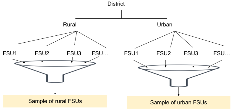
- (Random?) Sample from group of First Stage Units (FSU)
- Each FSU usually has a population within a range
- e.g. census geographies (census block, metropolitan statistical area, etc.)
- (Random?) Sample from group of First Stage Units (FSU)
- Stage 2
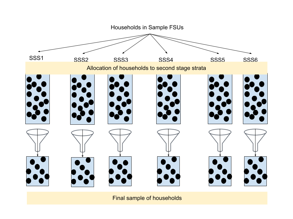
- All Second Stage Units (SSU) within each FSU are pooled together to create a population
- SSUs are the base geography unit you want to measure
- e.g. households
- Then each SSU is binned into Second Stage Strata (SSS) according to a characteristic or set of characteristics
- e.g. race, age, income level, education, etc.
- The SSS are stratified sampled
- All Second Stage Units (SSU) within each FSU are pooled together to create a population
Multi-Phase Sampling
- Instead of sampling units within each cluster like in mult-stage sampling, units are sampled from the union of all units within the selected clusters.
- Depending on the assigned probabilities and selection method, some multi-phase designs are strictly equivalent to multi-stage designs.
Systematic Sampling
- Steps
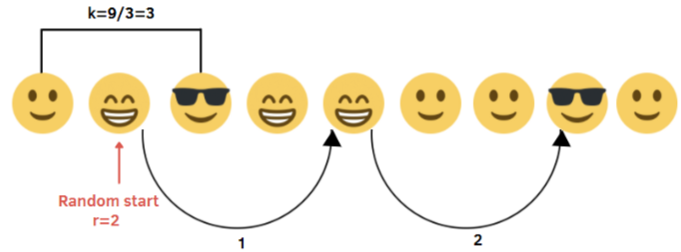
- After choosing a sample size, n, calculate the sampling interval k = N/n, where N is the population size
- In the example, we have 9 smiles and we want to obtain a sample of 3 units, then N = 9, n = 3 and k = 9/3 =3.
- Select a random starting point, r, which is a random integer between 1 and k: 1≤r≤k.
- In the example, r = 2, where 1≤r≤3.
- Once the first unit is selected, we take every following kth item to build the sample: r, r+k, r+2k , … , r+(n-1)k.
- After choosing a sample size, n, calculate the sampling interval k = N/n, where N is the population size
- Advantages:
- The random selection is applied only on the first item, while the rest of the items selected depend on the position of the first item and a fixed interval at which items are picked.
- Disadvantages:
- If the list of the population elements presents a determined order, there is the risk of obtaining a non-representative sample
Non-Probabilistic Sampling Methods
- Misc
- Mostly used when probabilistic methods aren’t possible due to rarity or difficulty in obtaining a representative sample of the population being studied or cost constraints of the experiment
- Packages
- {nonprobsvy} - Inference Based on Non-Probability Samples and {jointCalib} - A Joint Calibration of Totals and Quantiles
- Papers:
- Utilizes a method of joint calibration for totals and quantiles to extend existing inference methods for non-probability samples, such as inverse probability weighting, mass imputation and doubly robust estimators which produces results that are more robust against model mis-specification and helps to reduce bias and improve estimation efficiency.
- {nonprobsvy} - Inference Based on Non-Probability Samples and {jointCalib} - A Joint Calibration of Totals and Quantiles
- Quota Sampling
- Similar to Stratified Sampling (see Probabilistic Sampling Methods) except:
- Each stratum’s sample size is called its quota
- Each stratum’s sample size takes into account its distribution in the whole population.
- Example: If 80% of the population are males, then 80% of the sample should be males.
- Within each stratum’s quota, the interviewer is free to choose the participants to interview.
- This seems to be the main difference
- Advantages:
- It’s time and cost-effective, in particular with respect to the stratified sampling.
- Disadvantages:
- The results can be distorted due to the discretion of the interviewers or the non-response bias
- The quota sample can produce a selection bias
- Similar to Stratified Sampling (see Probabilistic Sampling Methods) except:
- Judgemental Sampling (aka Purposive Sampling)
- The researcher selects the participants because he believes they are representative of the population
- Useful when there is only a limited number of people with specific traits
- Advantages:
- It’s time and cost-effective
- It’s suitable to study a certain cultural domain, where the knowledge of an expert is needed
- Disadvantages:
- It can lead to a high selection bias the bigger is the gap between the researcher’s knowledge and the actual situation of the population
- The researcher selects the participants because he believes they are representative of the population
- Convenience Sampling
- The researcher chooses anyone that is “convenient” to him, i.e. people that are immediately available to answer the questions, without any specific criteria
- Usually volunteers
- Advantages:
- It’s very cheap and fast
- Disadvantages:
- It leads to a non-representative sample
- The researcher chooses anyone that is “convenient” to him, i.e. people that are immediately available to answer the questions, without any specific criteria
- Snowball Sampling
- The researcher asks already recruited people to identify other potential participants, and so on
- Useful for rare populations, for which it’s not possible to have the list of the population or it’s difficult to locate the population.
- e.g. illegal immigrants
- Useful for rare populations, for which it’s not possible to have the list of the population or it’s difficult to locate the population.
- Advantages:
- It’s useful for market studies or researches about delicate topics.
- Disadvantages:
- The sample may be non-representative since it’s not random, but depends on the people contacted directly or indirectly by the researcher
- It’s time-consuming
- The researcher asks already recruited people to identify other potential participants, and so on