Mixed Effects

Misc

Packages
- {performance} - Utilities for computing indices of model quality and goodness of fit.
  - Metrics such as R-squared (R²), root mean squared error (RMSE), intraclass correlation coefficient (ICC), etc.
  - Checks for overdispersion, zero-inflation, convergence, or singularity.
- {ggResidpanel} - Standard residual plots with appropriate residual types depending on whether it’s a glm or lm type of model. Uses {ggplot2}
  - Has convenience function for plotting residuals vs predictors
  - Natively supports models of type “lm”, “glm”, “lme”, “lmer”, “glmer”, and “lmerTest” out of the box
  - Can support other models types with resid_auxpanel if you want to supply your own residuals and fitted/predicted values.

Convergence Issues

See ?lme4::convergence
Gist of Checks (Choe)
- Set a more lenient tolerance for the gradient
- Turn off gradient optimization (?)
- Use stricter precision
- Restart the fit from the reported optimum, or from a point perturbed slightly away from the reported optimum

Test all optimizers: To assess whether convergence warnings render the results invalid, or to the contrary, the results can be deemed valid in spite of the warnings, Bates et al. (2023) suggest refitting models affected by convergence warnings with a variety of optimizers. (article)

If all optimizers converge to values that are practically equivalent, then consider the convergence warnings to be false positives.

Example: {lme4}

library(lme4)
library(dfoptim)
library(optimx)

fit <- lmer(fatigue ~ spin * reg + (1|ID),
           data = testdata, REML = TRUE)

# Refit model using all available algorithms
multi_fit <- allFit(fit)
#> bobyqa : [OK]
#> Nelder_Mead : [OK]
#> nlminbwrap : [OK]
#> nmkbw : [OK]
#> optimx.L-BFGS-B : [OK]
#> nloptwrap.NLOPT_LN_NELDERMEAD : [OK]
#> nloptwrap.NLOPT_LN_BOBYQA : [OK]
summary(multi_fit)$fixef
#>                               (Intercept)      spin       reg  spin:reg
#> bobyqa                          -2.975678 0.5926561 0.1437204 0.1834016
#> Nelder_Mead                     -2.975675 0.5926559 0.1437202 0.1834016
#> nlminbwrap                      -2.975677 0.5926560 0.1437203 0.1834016
#> nmkbw                           -2.975678 0.5926561 0.1437204 0.1834016
#> optimx.L-BFGS-B                 -2.975680 0.5926562 0.1437205 0.1834016
#> nloptwrap.NLOPT_LN_NELDERMEAD   -2.975666 0.5926552 0.1437196 0.1834017
#> nloptwrap.NLOPT_LN_BOBYQA       -2.975678 0.5926561 0.1437204 0.1834016

{lme4::allfit} requires the other two packages to fit all available optimizers
Article also has a custom plotting function to visually compare the results

Metrics

Also see
- Mixed Effects, BMLR >> Ch.8 >> Model Building Workflow >> Unconditional Means for an ICC example
- Mixed Effects, General >> Examples >> Example 1 >> Varying Intercepts for an ICC example
Restricted Maximum Likelihood (REML)
- It is a form of the likelihood function that accounts for the loss of degrees of freedom due to the estimation of the fixed effects parameters
- The REML criterion is minimized during the model estimation process, and the estimation algorithm iterates until it converges to a point where the REML criterion cannot be further minimized. The value of the REML criterion at this convergence point is reported in the model summary.
- A lower value is better, but the REML criterion value itself is not directly interpretable. it is mainly used for comparing the relative fit of different models to the same data.
- Does not account for model complexity or the principle of parsimony, so it should be used in conjunction with domain knowledge and other metrics.
Check Degrees of Freedom (DOF) in Fixed Effects Estimates
- The degrees of freedom for the estimates should be close to the number of subjects (aka units)
- Large degrees of freedom in comparison to the number of subjects indicates a misspecification of the model. (e.g. 60 subjects and dofs are close to the number of observations)
  - Degrees of Freedom that are less than then number of subjects are fine and could be due to substantially imbalanced numbers of observations among the subjects.
- Also papers should report the dofs.
- Example
```
library(lmerTest)
data("sleepstudy")
lmer_mod <- 
  lmer(Reaction ~ 1 + Days + (1 + Days | Subject),
       sleepstudy,
       REML = 0)
summary(lmer_mod)

#> Fixed effects:
#>             Estimate Std. Error      df t value Pr(>|t|)    
#> (Intercept)  251.405      6.632  18.001  37.907  < 2e-16 ***
#> Days          10.467      1.502  18.000   6.968 1.65e-06 ***

lmer_mod2 <- 
  lmer(Reaction ~ 1 + Days + (1 | Subject),
       sleepstudy,
       REML = 0)
summary(lmer_mod2)
#> Fixed effects:
#>             Estimate Std. Error       df t value Pr(>|t|)    
#> (Intercept) 251.4051     9.5062  24.4905   26.45   <2e-16 ***
#> Days         10.4673     0.8017 162.0000   13.06   <2e-16 ***
```
  - There are 18 subjects, so the first model is a well-specified model
  - The dof spikes to 162 for the Days fixed effect which is close to the number of total observations at 180. This indicates a misspecified model.
    - The 24.4905 is actually okay for the intercept.
  - Note that you need to used {lmerTest} and not {lme4} to fit the model in order to get the dofs and pvals. Although there’s probably a helper function in {lmerTest} since it loads {lme4} that will give the same results if you fit the model using {lme4}
InterClass Coefficient (ICC): The proportion of variation that is between-cases

\[ \rho = \frac{\sigma_0}{\sigma_0 + \sigma_\epsilon} \]
- Where $\sigma_0$ is the between-case variance and $\sigma_\epsilon$ is the within-case variance.
- 1-ICC is the proportion of variation within cases
  - Although {sjPlot::tab_model} does compute a ICC for varying slopes models
- Statistical power is a function of ICC (article)
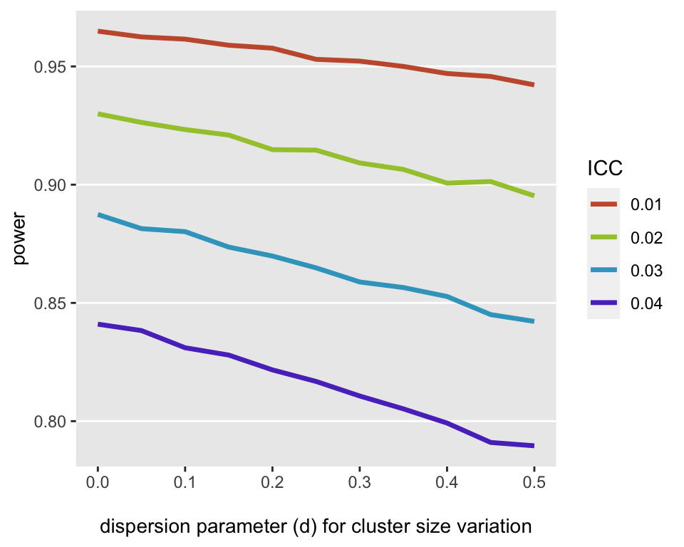
  - Both higher ICCs and cluster size variability lead to reduced power
  - The dispersion parameter is a parameter used in the data simulation
- Guideline: ICC > 0.1 is generally accepted as the minimal threshold for justifying the use of Mixed Effects Model
- Example 1: {sjPlot}
```
library(sjPlot)
tab_model(lme_fit)
```
  - Might need {lmerTest} loaded to get coefficient pvals
  - Also calculates two R² values
    - Marginal: proportion of variance explained by the fixed effects only
    - Conditional: proportion of variance explained by the fixed effects and random effects
- Example 2: {performance}
```
data("stroop", package = "afex")
stroop_sub <- subset(stroop, !is.na(rt))

stroop_agg <- 
 stroop_sub |> 
 summarize(mean_rt = mean(rt),
           .by = c("pno", "congruency", "condition"))

MLM <- lmerTest::lmer(rt ~ congruency * condition + (1 | pno),
                      data = stroop_agg)
performance::icc(MLM)
#> # Intraclass Correlation Coefficient
#> 
#>     Adjusted ICC: 0.752
#>   Unadjusted ICC: 0.632
```
  - Adjusted ICC only relates to the random effects
  - Unadjusted ICC takes the random effects and fixed effects variances into account, more precisely, the fixed effects variance is added to the denominator of the formula to calculate the ICC
  - Don’t pay attention to the aggregation. It was done just to illustrate a point about the necessity of varying slopes even in cases where there is no repeated measure
R², AICc, BICc
- Packages
  - {greybox::AICc} or {greybox::BICc} for corrected versions of the information criterion metrics. Supposed to work on any model with logLik and nobs methods
    - Lower is Better (which is the model that minimizes the information loss)
  - {glmm.hp} - Hierarchical Partitioning of Marginal R² for Generalized Mixed-Effect Models
    - Calculates individual contributions of each predictor (fixed effects) towards marginal R²
- Example: From ICC >> Example 2
```
performance::r2(MLM)
#> # R2 for Mixed Models
#> 
#>   Conditional R2: 0.792
#>      Marginal R2: 0.161
greybox::AICc(MLM)
#> [1] -5910.074
greybox::BICc(MLM)
#> [1] -5904.154
```
  - Nakagawa’s R² is used
  - Conditional R²: Takes both the fixed and random effects into account.
  - Marginal R²: Considers only the variance of the fixed effects.

Residuals

Misc
- {DHARMa} - Built for Mixed Effects Models for count distributions but also handles lm, glm (poisson) and MASS::glm.nb (neg.bin)
Binned Residuals
- It is not useful to plot the raw residuals, so examine binned residual plots
- Misc
  - {arm} will mask some {tidyverse} functions, so don’t load whole package
- Look for :
  - Patterns
  - Nonlinear trend may be indication that squared term or log transformation of predictor variable required
  - If bins have average residuals with large magnitude
  - Look at averages of other predictor variables across bins
  - Interaction may be required if large magnitude residuals correspond to certain combinations of predictor variables
- Process
  1. Extract raw residuals
    - Include type.residuals = "response" in the broom::augment function to get the raw residuals
  2. Order observations either by the values of the predicted probabilities (or by numeric predictor variable)
  3. Use the ordered data to create g bins of approximately equal size.
    - Default value: g = sqrt(n)
  4. Calculate average residual value in each bin
  5. Plot average residuals vs. average predicted probability (or average predictor value)
- Example: vs Predicted Values
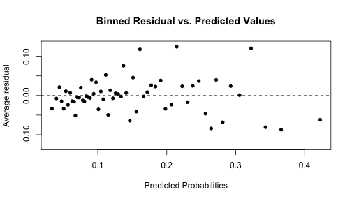
```
arm::binnedplot(x = risk_m_aug$.fitted, y = risk_m_aug$.resid,
                xlab = "Predicted Probabilities",
                main = "Binned Residual vs. Predicted Values",
                col.int = FALSE)
```
- Example: vs Predictor
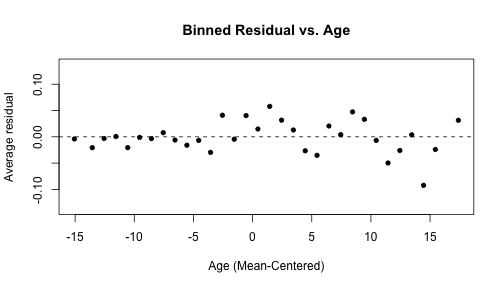
```
arm::binnedplot(x = risk_m_aug$ageCent,
                y = risk_m_aug$.resid,
                col.int = FALSE,
                xlab = "Age (Mean-Centered)",
                main = "Binned Residual vs. Age")
```
Check that residuals have mean zero: mean(resid(mod))

Check that residuals for each level of categorical have mean zero

risk_m_aug %>%
  group_by(currentSmoker) %>%
  summarise(mean_resid = mean(.resid))

Check for normality.

# Normal Q-Q plot
qqnorm(resid(mod))
qqline(resid(mod))

Check normality per categorical variable level
- Example: 3 levels
```
## by level
par(mfrow=c(1,3))

qqnorm(resid(mod)[1:6])
qqline(resid(mod)[1:6])

qqnorm(resid(mod)[7:12])
qqline(resid(mod)[7:12])

qqnorm(resid(mod)[13:18])
qqline(resid(mod)[13:18])
```
  - Data should be sorted by random variable level before modeling. Otherwise you could column bind the residuals to the original data. Then, group by random variable and make q-q plots for each group

Examples

Example 1: {performance}l Varying Intercepts, Varying Slopes
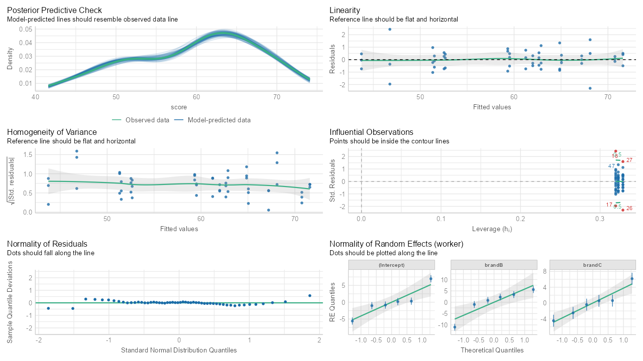
```
library(performance); 
library(lmerTest)
library(dplyr)

data(Machines, package = "nlme")

machines <- Machines |> 
  mutate(Worker = factor(Worker, 
                         levels = 1:6, 
                         ordered = FALSE)) |> 
  rename(worker = Worker, brand = Machine) |> 
  group_by(brand, worker) |> 
  mutate(avg_score = mean(score)) 

mod_bw_si <- 
  lmer(score ~ brand + (1 + brand | worker),
       data = machines)

check_model(mod_bw_si)

model_performance(mod_bw_si)
# Indices of model performance

#> AIC     |    AICc |     BIC | R2 (cond.) | R2 (marg.) |   ICC |  RMSE | Sigma
#> -----------------------------------------------------------------------------
#> 228.311 | 233.427 | 248.201 |      0.987 |      0.468 | 0.975 | 0.791 | 0.962
```
- Instructions for interpeting each plot are in the subtitles
- Homogeneity of Variance shows a little bit of heterskedacity with the gentle slope from left to right.
- The Influential Observations doesn’t have any “contours,” but I assume the red points are the influential observations to be interested in.
- Normality of Residuals shows a bit of an issue in the right tail and maybe a little something in the left tail.
- The normality of REs by worker show all the point estimates within range with a few CIs outside.
- Overall this looks like a pretty good fit to me. Perhaps examine the influential observations. Also, the outcome variable shows some bi-modal-ness and left-skew, so maybe something could be done to model that better.
- Most of the metrics are for model comparison. ICC is over 0.10, R²(cond) is high so the modeling of the random effects is good. But R² (marg) is quite low, so perhaps some transformations, interactions, splines, or just adding more adjustment variables can be raise that.
Example 2: {ggResidpanel}; Residuals vs Predictors
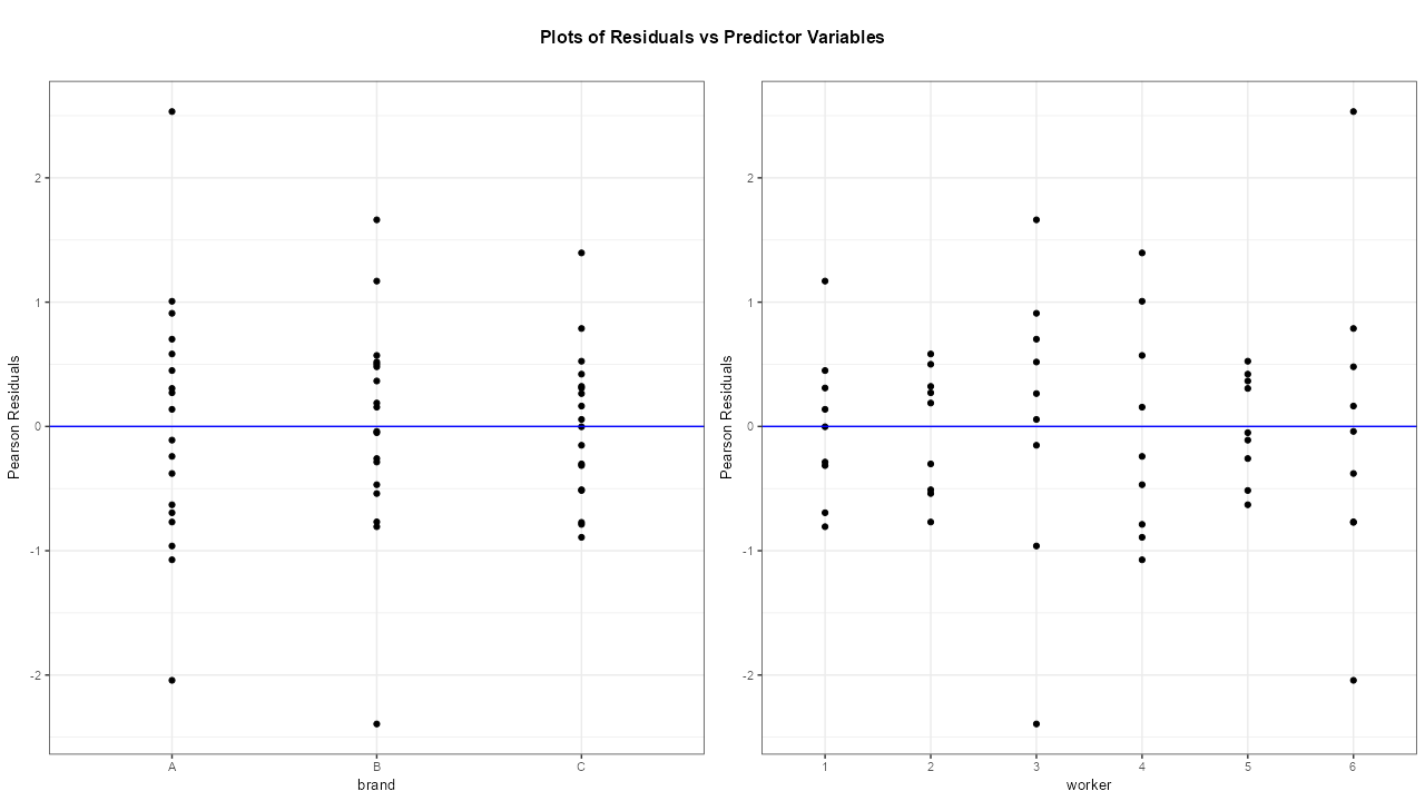
```
ggResidpanel::resid_xpanel(mod_bw_si)
```
- Model from Example 1
- There are some large residuals in brands A and B and also for workers 3 and 6