Linear Algebra

Misc

Packages
- {gghinton} - {ggplot2} extension for drawing Hinton diagrams,
  - A visualization technique for numerical matrices in which the area of each square is proportional to the magnitude of the corresponding entry
  - Useful for visualising PCA weight matrices, correlation matrices, and transition matrices.
- {GPUmatrix} (Github) - Mimics the behavior of {Matrix} and extends R to use the GPU for computations. It includes single(FP32) and double(FP64) precision data types, and provides support for sparse matrices. Able to use Tensorflow or Torch.
- {Matrix} - A rich hierarchy of sparse and dense matrix classes, including general, symmetric, triangular, and diagonal matrices with numeric, logical, or pattern entries.
  - Efficient methods for operating on such matrices, often wrapping the ‘BLAS’, ‘LAPACK’, and ‘SuiteSparse’ libraries
- {sparsevctrs} - Sparse Vectors for Use in Data Frames or Tibbles
  - Sparse matrices are not great for data in general, or at least not until the very end, when mathematical calculations occur.
  - Some computational tools for calculations use sparse matrices, specifically the Matrix package and some modeling packages (e.g., xgboost, glmnet, etc.).
  - A sparse representation of data that allows us to use modern data manipulation interfaces, keeps memory overhead low, and can be efficiently converted to a more primitive matrix format so that we can let Matrix and other packages do what they do best.
- {quickr} - R to Fortran Transpiler
  - Only atomic vectors, matrices, and array are currently supported: integer, double, logical, and complex.
  - The return value must be an atomic array (e.g., not a list)
  - Only a subset of R’s vocabulary is currently supported.
    #> [1] != %% %/% & && ( * #> [8] + - / : < <- <= #> [15] = == > >= Fortran [ [<- #> [22] ^ c cat cbind character declare double #> [29] for if ifelse integer length logical matrix #> [36] max min numeric print prod raw seq #> [43] sum which.max which.min { | ||

Resources

Crash Course in Matrix Algebra: A Refresher on Matrix Algebra for Econometricians with Implementation in R
See Matrix Cookbook pdf in R >> Documents >> Mathematics
- derivatives, inverses, statistics, probability, etc.
Link - A lot of matrix properties as related to regression, covariance, coefficients, etc.
EBOOK statistical linear algebra: basics, transformations, decompositions, linear systems, regression - Matrix Algebra for Educational Scientists
Video Course: Linear Algebra for Data Science - Basics, Least Squares, Covariance, Regression, PCA, SVD
Powered by Linear Algebra: The central role of matrices and vector spaces in data science by Matloff
- Delta Method, Regularized Regression, PCA, SVD, Attention

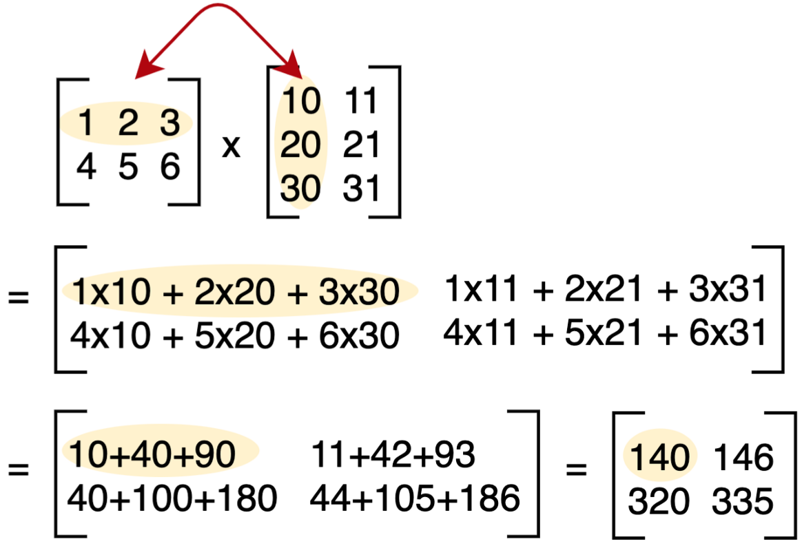
Matrix Multiplication

Matrix Algebra

An expected value equation (VC stands for variance-covariance in example) multiplied by a matrix, C.
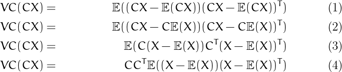
- C is factored out of an expected value as C
- C is factored out of a transpose as CT

Factorization

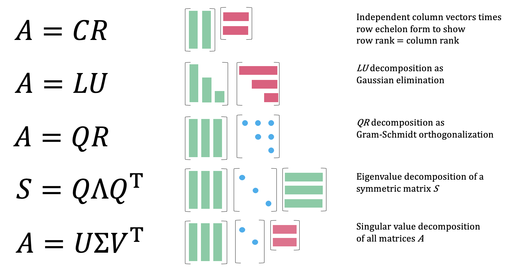
\(A = CR\) (Column-Row)
- Factors A into a matrix \(C\) of linearly independent columns of \(A\), and \(R\), the row echelon form
- Proves that row rank equals column rank
- Use cases:
  - Theoretical and pedagogical tool to understand rank and linear independence
\(A = LU\) (LU Decomposition)
- Splits \(A\) into a lower triangular matrix \(L\) and upper triangular matrix \(U\) via Gaussian elimination
- Use cases:
  - Solving systems of linear equations \(Ax = b\)
  - Computing determinants
  - Matrix inversion
  - Numerical software libraries such as LAPACK
\(A = QR\) (QR Decomposition)
- Factors \(A\) into an orthogonal matrix \(Q\) and upper triangular matrix \(R\) via Gram-Schmidt orthogonalization
- Use cases:
  - Solving least squares problems
  - Computing eigenvalues iteratively via the QR algorithm
  - Numerically stable solutions to linear systems
\(S = Q\Lambda Q^T\) (Eigenvalue Decomposition)
- Decomposes a symmetric matrix \(S\) into its eigenvectors (columns of \(Q\)) and a diagonal matrix \(\Lambda\) of eigenvalues
- Use cases:
  - Principal Component Analysis (PCA)
  - Quantum mechanics
  - Solving differential equations
  - Understanding the geometry of linear transformations
\(A = U\Sigma V^T\) (Singular Value Decomposition (SVD))
- The most general factorization, works on any matrix; \(U\) and \(V\) are orthogonal matrices of singular vectors, \(\Sigma\) is diagonal with singular values
- Use cases:
  - Dimensionality reduction
  - Image compression
  - Recommender systems
  - Pseudoinverse computation
  - Low-rank approximations
\(A = WH\) (Non-Negative Matrix Factorization (NMF))
- Also see Algorithms, Recommender >> Collaborative Filtering >> Non-Negative Matrix Factorization (NMF)
- Factors a non-negative matrix \(A\) into two non-negative matrices \(W\) (basis or contribution matrix) and \(H\) (coefficient or composition matrix)
- Unlike other factorizations, the non-negativity constraint produces additive, parts-based representations that are often more interpretable
- No closed-form solution; computed iteratively via multiplicative update rules or gradient descent
- Use cases:
  - Topic modeling in natural language processing (identifying themes in document collections)
  - Image decomposition and facial feature recognition
  - Audio source separation (e.g. isolating instruments in a mixed recording)
  - Bioinformatics (e.g. gene expression analysis)
  - Recommender systems (e.g. user-item matrix factorization)

Methods

The Moore-Penrose Inverse

The Moore-Penrose inverse, often denoted as \(A^+\), is a generalization of the ordinary matrix inverse that applies to any matrix, even those that are singular (non-invertible) or rectangular. It was independently developed by E.H. Moore and Roger Penrose.
Generalized Inverse
- Unlike a regular inverse, which only exists for square, non-singular matrices, the Moore-Penrose inverse exists for all matrices. This is incredibly useful in situations where you have more equations than unknowns (overdetermined systems) or fewer equations than unknowns (underdetermined systems), or when your matrix is singular.
Four Penrose Conditions
- The Moore-Penrose inverse \(A^+\) of a matrix \(A\) is uniquely defined by four conditions:
  1. \(A A^+ A = A\)
  2. \(A^+ A A^+ = A^+\)
  3. \((A A^+)^T = A A^+\)
  4. \((A^+ A)^T = A^+ A\)
Least Squares Solution
- One of its most important applications is in finding the “best fit” (least squares) solution to a system of linear equations \(Ax = b\). When an exact solution doesn’t exist (e.g., in overdetermined systems), the Moore-Penrose inverse provides the \(x\) that minimizes the Euclidean norm of the residual error, \(\|Ax - b\|^2\). The solution is given by \(x = A^+ b\). If there are multiple solutions (e.g., in underdetermined systems), it provides the solution with the minimum Euclidean norm \(\|x\|^2\).
Computation
- The most common and robust method for computing the Moore-Penrose inverse is through Singular Value Decomposition (SVD). If \(A = U \Sigma V^T\) is the SVD of \(A\), then \(A^+ = V \Sigma^+ U^T\), where \(\Sigma^+\) is obtained by taking the reciprocal of the non-zero singular values in \(\Sigma\) and transposing the resulting matrix.

Unmixing

The process of decomposing a mixed signal or observation into its constituent pure components (called endmembers) and determining how much each component contributes to the mixture (called abundances).
Resources
It relates naturally to NMF because the non-negativity constraint maps directly onto physical reality — most real-world mixtures (light, sound, chemicals, etc.) cannot have negative components.
- The basis matrix \(W\) holds the pure endmember profiles and the coefficient matrix \(H\) holds the mixing proportions.
- Because both are constrained to be non-negative, the result is interpretable as a physically meaningful additive mixture — something that methods like PCA or SVD cannot guarantee, since they allow negative values that have no clear real-world interpretation.
Use Cases:
- Hyperspectral imaging - A pixel in a satellite image might contain a mixture of soil, vegetation, and water. Unmixing identifies the pure spectral signatures (W) and their proportions (H) in each pixel
- Audio - A recording of multiple instruments is a mixture; unmixing recovers the individual sources
- Chemometrics - A chemical sample measured by spectroscopy may contain multiple substances; unmixing recovers the pure spectra and concentrations
- Neuroscience - Brain imaging signals are mixtures of activity from different neural populations; unmixing separates them
Adjustments must be made to the \(W\) and \(H\) matrices:
- Row-standardize the \(W\) matrix: divide each entry in the matrix by the corresponding row sum.
- Multiply the \(H\) matrix by the ratio of the column sums of the \(W\) matrix before and after row-standardization.

Specialty Matrices

Notes from Derivatives, Gradients, Jacobians and Hessians – Oh My!
Jacobian

\[ \begin{align} &v, w = f(x, y, z) \\ &\mathbb{J} = \begin{bmatrix} \frac{\partial v}{\partial x} & \frac{\partial v}{\partial y} & \frac{\partial v}{\partial z} \\ \frac{\partial w}{\partial x} & \frac{\partial w}{\partial y} & \frac{\partial w}{\partial z} \end{bmatrix} \end{align} \]
- Also see (Video) The Jacobian : Data Science Basics for it’s usage in ML
- The gradient is calculated for v and the gradient is calculated for w. Then, the result is put into matrix.
- At a specific point in space (of whatever space the input parameters are in), it tells you how the space is warped in that location – like how much it is rotated and squished.
- The determinent of the Jacobian:
  - \(\gt 1\) : Things get bigger
  - \(\lt 1\) but \(\gt 0\) : Things get smaller
  - \(\lt 0\) : Things get flipped
  - \(0\) : Things get squished to a point, and the matrix is not invertible
Hessian
\[ \begin{align} &w = f(x, y, z) \\ &\mathbb{H} = \begin{bmatrix} \frac{\partial^2 w}{\partial x^2} & \frac{\partial^2 w}{\partial xy} & \frac{\partial^2 w}{\partial xz} \\ \frac{\partial^2 w}{\partial yx} & \frac{\partial^2 w}{\partial y^2} & \frac{\partial^2 w}{\partial yz} \\ \frac{\partial^2 w}{\partial zx} & \frac{\partial^2 w}{\partial zy} & \frac{\partial^2 w}{\partial z^2} \end{bmatrix} \end{align} \]
- See
- Taking the second derivative is taking partial derivatives (3 total, 1 w.r.t. each variable) of each partial derivative (3 total, 1 w.r.t. each variable) for a grand total of 9 partial derivatives.

R

drop = TRUE (default): If TRUE the result is coerced to the lowest possible dimension

This only works for extracting elements, not for the replacement

Example:

(m <- matrix(1:3, nrow = 3))
#>      [,1]
#> [1,]    1
#> [2,]    2
#> [3,]    3

m[1:2,]
#> [1] 1 2

class(m[1:2,])
#> [1] "integer"

m[1:2, , drop = FALSE]
#>      [,1]
#> [1,]    1
#> [2,]    2

class(m[1:2, , drop = FALSE])
#> [1] "matrix" "array" 

rowSums(m[1:2,])
#> Error in rowSums(m[1:2, ]) : 
#>   'x' must be an array of at least two dimensions

rowSums(m[1:2, , drop = FALSE])
#> [1] 1 2

Example: Difference between a column and a lag

from blah blah

Each column is a time step (e.g. day 1, day 2, day 3, etc.)

set.seed(2026)

(Y <- matrix(sample(1:18, 18), nrow = 3))
#>      [,1] [,2] [,3] [,4] [,5] [,6]
#> [1,]    1   15    4    2   14    9
#> [2,]    6   11    5    8   18    7
#> [3,]   13   12   10    3   16   17

T <- ncol(Y)
u <- 1 # lag 1

# cols 1:5
Y[, 1:(T - u), drop = FALSE] 
#>      [,1] [,2] [,3] [,4] [,5]
#> [1,]    1   15    4    2   14
#> [2,]    6   11    5    8   18
#> [3,]   13   12   10    3   16

# cols 2:6
Y[, (1 + u):T, drop = FALSE]
#>      [,1] [,2] [,3] [,4] [,5]
#> [1,]   15    4    2   14    9
#> [2,]   11    5    8   18    7
#> [3,]   12   10    3   16   17

# difference
Y[, 1:(T - u), drop = FALSE] -
  Y[, (1 + u):T, drop = FALSE]
#>      [,1] [,2] [,3] [,4] [,5]
#> [1,]  -14   11    2  -12    5
#> [2,]   -5    6   -3  -10   11
#> [3,]    1    2    7  -13   -1

Column 2 is subtracted from column 1. Column 3 is subtracted from column 2 and so on.
T is number of columns which is the maximum number of lags we can calculate the difference for.

u <- 2 # lag 2

# cols 1:4
Y[, 1:(T - u), drop = FALSE] 
#>      [,1] [,2] [,3] [,4]
#> [1,]    1   15    4    2
#> [2,]    6   11    5    8
#> [3,]   13   12   10    3

# cols 3:6
Y[, (1 + u):T, drop = FALSE]
#>      [,1] [,2] [,3] [,4]
#> [1,]    4    2   14    9
#> [2,]    5    8   18    7
#> [3,]   10    3   16   17

# difference
Y[, 1:(T - u), drop = FALSE] -
  Y[, (1 + u):T, drop = FALSE]
#>      [,1] [,2] [,3] [,4]
#> [1,]   -3   13  -10   -7
#> [2,]    1    3  -13    1
#> [3,]    3    9   -6  -14

With the second lag, the total number of columns for each submatrix is 2 fewer than the original total. (It was 1 fewer for lag 1)
- This explains why the number of columns is the maximum number of lags

u <- 3 # lag 3

# cols 1:3
Y[, 1:(T - u), drop = FALSE] 
#>      [,1] [,2] [,3]
#> [1,]    1   15    4
#> [2,]    6   11    5
#> [3,]   13   12   10

# cols 4:6
Y[, (1 + u):T, drop = FALSE]
#>      [,1] [,2] [,3]
#> [1,]    2   14    9
#> [2,]    8   18    7
#> [3,]    3   16   17

# difference
Y[, 1:(T - u), drop = FALSE] -
  Y[, (1 + u):T, drop = FALSE]
#>      [,1] [,2] [,3]
#> [1,]   -1    1   -5
#> [2,]   -2   -7   -2
#> [3,]   10   -4   -7

Y[2,2] <- NA
Y
#>      [,1] [,2] [,3] [,4] [,5] [,6]
#> [1,]    1   15    4    2   14    9
#> [2,]    6   NA    5    8   18    7
#> [3,]   13   12   10    3   16   17 

u <- 1 # lag 1

Y[, 1:(T - u), drop = FALSE] 
#>      [,1] [,2] [,3] [,4] [,5]
#> [1,]    1   15    4    2   14
#> [2,]    6   NA    5    8   18
#> [3,]   13   12   10    3   16

Y[, (1 + u):T, drop = FALSE]
#>      [,1] [,2] [,3] [,4] [,5]
#> [1,]   15    4    2   14    9
#> [2,]   NA    5    8   18    7
#> [3,]   12   10    3   16   17

(diff <- Y[, 1:(T - u), drop = FALSE] - 
  Y[, (1 + u):T, drop = FALSE])
#>      [,1] [,2] [,3] [,4] [,5]
#> [1,]  -14   11    2  -12    5
#> [2,]   NA   NA   -3  -10   11
#> [3,]    1    2    7  -13   -1

diff^2 
#>      [,1] [,2] [,3] [,4] [,5]
#> [1,]  196  121    4  144   25
#> [2,]   NA   NA    9  100  121
#> [3,]    1    4   49  169    1

So NA - number or vice-versa is NA, and squaring the matrix shows that NA² is NA.