Interactions
Misc
- Also see
- EDA, General >> Interactions
- Post-Hoc Analysis, emmeans >> Interactions
- More {marginaleffects} and {emmeans} examples
- Partial Residuals
- Introduction: Adding Partial Residuals to Marginal Effects Plots for detecting interactions using residuals of a regression model.
- Exploring interactions with continuous predictors in regression models
- Causal Inference, Moderation Analysis
- Diagnostics, Model Agnostic >>
- DALEX >> Instance Level >> Break-Down >> Example: Assume Interactions
- DALEX >> Instance Level >> Ceteris Paribus (CP)
- DALEX >> Dataset Level >> Partial Dependence Plots (PDPs)
- SHAP >> Interactions and {treeshap}
- IML >> Interaction PDP and H-Statistic
- Packages
- {APCinteraction} - A nonparametric R package for detecting interactions in two-way ANOVA designs with balanced replication using all possible crossed comparisons (APC).
- Provides 180 pre-computed null distributions (100,000 simulations each) for the APCSSA and APCSSM nonparametric interaction test statistics.
- {interactions} - Tools for the analysis and interpretation of statistical interactions in regression models.
- Features
- Simple Slopes Analysis
- Calculation of Johnson-Neyman intervals
- Visualization of predicted and observed values using {ggplot2}
- Supported Models:
glm,lm, {survey}, {lme4}, {rstanarm}, and {brms}
- Features
- {InteractionPoweR} - Power Analyses for Interaction Effects in Cross-Sectional Regressions
- Tests the interaction of two or three independent variables on a single dependent variable.
- Includes options for correlated interacting variables and specifying variable reliability.
- Two-way interactions can include continuous, binary, or ordinal variables.
- {ixsurface} - Interactive 3D Surface Plots for Multi-Factor Interaction Visualization
- Supports continuous, categorical, and mixed factor designs with automatic binning for continuous conditioning variables.
- {marginaleffects}
- Book - Interpretation, tons of examples; python and r code
- Experiments, Observational data, Causal inference with G-Computation, Machine learning models, Bayesian modeling, Multilevel regression with post-stratification (MRP), Missing data, Matching, Inverse probability weighting, Conformal prediction
- Paper: How to Interpret Statistical Models Using marginaleffects for R and Python
- Supported Models, Adding a model to the package
- marginaleffects skill for both R and Python and both Claude and Codex
- Functions
predictions- Ffamily of functions that can compute and plot predictions on different scales (aka “fitted values”). It can also aggregate or marginalize predicted values, over a whole dataset or by subgroups (i.e., “marginal means”)comparisons- Family of functions that can compute and plot relationships between two or more predictions. This allows users to report many of the most common quantities of interest in statistical analyses: contrasts, differences, risk ratios, odds ratios, lift, or even arbitrary user-defined functions of two predictions.slopes- Family of functions that can compute and plot partial derivatives of the outcome equation. In the econometrics tradition, researchers typically call these slopes “marginal effects,” where the term “marginal” refers to a “small change.” Analysts can easily evaluate these derivatives at different points in the predictor space, they can aggregate unit-level estimates to produce global summaries, and they conduct hypothesis tests to compare different slopes- Slopes are defined as derivatives, that is, in terms of an infinitesimal change in X, they can only be constructed for continuous numeric predictors.
avg_slopes- Calculates the average marginal effect (AME) by plugging each row of the original data into the model, generating predictions and instantaneous slopes for each row, and then averaging the estimate column
inferences- Bootstrap, Conformal, and Simulation-Based Inference- Apply this function to a marginaleffects object to change the inferential method used to compute uncertainty estimates.
plot_*- variables is the variable whose slope, mean will be on the Y-axis
- conditon is a vector or list of variables you want to stratify by
- The first variable listed will be on the X-axis, so you could, untraditionally have slope and x-axis variable be different.
- The second variable is a group by variable
- Book - Interpretation, tons of examples; python and r code
- {mlmoderator} - Provides a unified workflow for probing, plotting, and assessing the robustness of cross-level interaction effects in two-level mixed-effects models fitted with {lme4}
- {modelbased} (JOSS) - Easystats package built on top of marginaleffects and emmeans
- Successor package to {ggeffects}
- modelbased package for plotting interactions - Basic example of 2-way interaction in a poisson model
- {regress3d} - Plots regression surfaces and marginal effects in three dimensions.
- {simpr.interaction} - Analytically calculate parameters for the simulation of moderated multiple regression, based on the correlations among the predictors and outcome and the reliability of predictors.
- {unityForest} - Improving Interaction Modeling and Interpretability in Random Forests
- Currently, only classification is supported
- A random forest variant designed to better take covariates with purely interaction-based effects into account, including interactions for which none of the involved covariates exhibits a marginal effect.
- Facilitates the identification and interpretation of (marginal or interactive) effects
- Includes unity variable importance and covariate-representative tree roots (CRTRs) that provide interpretable visualizations of these conditions
- {APCinteraction} - A nonparametric R package for detecting interactions in two-way ANOVA designs with balanced replication using all possible crossed comparisons (APC).
- Resources
- R Syntax
- Operators (Equivalent Models)
- Colon (
:) -lm(y ~ x1 + x2 + x1:x2, data = df) - Asterisk (
*) -lm(y ~ x1 * x2, data = df)
- Colon (
- Combinations
- All main effects + all two-way interactions:
(x1 + x2 + x3 + x4)^2 - All main effects + all possible interactions (up to a three-way interaction):
x1 * x2 * x3 - Each variable in the first group (
x1,x2) interacts with each variable in the second group (x3,x4):(x1 + x2) * (x3 + x4)- i.e.
x1:x3,x1:x4andx2:x3,x2:x4
- i.e.
- All main effects + all two-way interactions:
- Operators (Equivalent Models)
- Stay away from polynomial interactions (unless there’s a theoretical/physical reason). High-order polynomial interactions like \(x^2y^2\) are notorious for instability at the boundaries of your data and lead to non-sensical predictions. (better to use splines instead)
- Rule of Thumb: In a balanced experiment, “you need 16 times the sample size to estimate an interaction than to estimate a main effect” in order to measure the interaction effect with the same precision as the main effect. There are contexts where it’s lower depending on the effect size. Gelman
- Selecting values of continuous predictors to use for calculating marginal effects
- Mean/Median and quantiles are popular choices
- Check if they’re multi-modal. If so, then the mean or median may not be a useful value to use for that variable when computing marginal effects.
- Modes for the distribution would be a suitable alternative.
- May also be useful to try to find intervals of values where there is no significant marginal effect.
- Using all combinations of values in the observed data to compute individual marginal effects and then taking the average will result in the average interaction effect
- Helpful in generating inferences about the whole population of interest instead of scenarios of interest or groups of interest
- Gelman and Hill: “Interactions can be important. In practice, inputs that have large main effects also tend to have large interactions with other inputs. (However, small main effects do not preclude the possibility of large interactions.)”
- We can probe or decompose interactions by asking the following research questions:
- What is the predicted Y given a particular X and W? (predicted value)
- What is relationship of X on Y at particular values of W? (simple slopes/effects)(marginal effects/predicted means)
- Is there a difference in the relationship of X on Y for different values of W? (comparing marginal effects)
- Predictors that are uncorrelated with each other still might have interaction effects on the response variable.
- Example: plant growth requires sunlight and rain. Without rain, sunlight will not increase growth and vice versa, but rain with sunlight does cause growth. This interaction effect exists even though amounts of sunlight and rain aren’t (very) correlated with each other
- Quadratic interaction example from {marginaleffects} vignette
- Dropping main effects
- For the cont x cat interaction, as long as you don’t drop a categorical main effect, I don’t think it affects the model. It may or may not reparameterize the interaction coefficients so they’re the marginal effects instead contrasts. (see article)
- e.g. for
admit ~ dept + gender:dept, the interpretation of an interaction coefficient might be something like male-female at dept A.
- e.g. for
- Whether it’s okay to drop the categorical variable, may depend on whether the main effects are significant or not
- Dropping a continuous main effects changes the model, so best not to ever do that in cat x cont or cont x cont interactions.
- Harrell said in a SO post that you should never do it.
- He had a link to blog post he’d written but the link was dead and there wasn’t anything in his RMS book.
- For the cont x cat interaction, as long as you don’t drop a categorical main effect, I don’t think it affects the model. It may or may not reparameterize the interaction coefficients so they’re the marginal effects instead contrasts. (see article)
- False linearity assumptions of main effects can inflate apparent interaction effects because interactions may be colinear with the omitted non-linear effect
- Interactions may also be non-linear, but shouldn’t also specify a nonlinear interaction w/smaller sample sizes
- With smaller sample sizes, make the main effect non-linear and the interaction component linear if the non-linear relationship is present between the interaction and outcome.
- Issue: Your interaction has a significant effect, but that effect disappears when you run a mixed effects model (See Gelman for ideas)
Terms
- Disordinal Interactions (aka crossover or antagonistic) - Interaction results whose lines do cross. (see fig in Ordinal Interactions)
- When an interaction is significant and “disordinal”, interpretation of main effects is likely to be misleading.
- To determine exactly which parts of the interaction are significant, the omnibus F test must be followed by more focused tests or comparisons.
- When an interaction is significant and “disordinal”, interpretation of main effects is likely to be misleading.
- Johnson-Neyman Interval - Tells you the range of values of the continuous moderator in which the slope of the predictor is significant vs. nonsignificant at a specified alpha level. (source)
- Instead of arbitrarily choosing points for continuous moderators, this method is a more statistically rigorous way to explore these effects.
- See {interactions}
- Marginal Effects - Partial derivatives of the regression equation with respect to each variable in the model for each unit (i.e. observation) in the data; average marginal effects are simply the mean of these unit-specific partial derivatives over some sample
- The Simple Slope or Simple Effect calculation is the same as the Marginal Effectcalculation from everything I’ve read. The only difference seems to be that the Marginal Effect can pertain a regression model without an interaction while Simple Slopes and Simple Effects are terms only used in describing effects in models with an interaction.
- i.e. the slope of the prediction function, measured at a specific value of the regressor
- In OLS regression with no interactions or higher-order term, the estimated slope coefficients are average marginal effects
- In other cases and for generalized linear models, the coefficients are NOT marginal effects at least not on the scale of the response variable
- Moderator Variable (MV) - A predictor that changes the relationship of a IV on the DV, and it can be continuous or categorical. Used in an interaction to estimate its effect on that relationship. (also see Causal Inference >> Moderation Analysis)
- Ordinal Interactions - Interaction results whose lines do not cross
.png)
- This looks like an EDA plot but also see OLS >> continuous:continuous >> Plot Simple Slopes
- Similar plot but for post-hoc analysis of a regression with an interaction
- Exponential Interaction: If the lines are not parallel but one line is steeper than the other, the interaction effect will be significant (i.e. detected) only if there’s enough statistical power.
- If the lines are exactly parallel, then there is no interaction effect
- This looks like an EDA plot but also see OLS >> continuous:continuous >> Plot Simple Slopes
- Simple Effect - When a Independent Variable interacts with a moderator variable (MV), it’s the differences in predicted values of the outcome variable at a particular level of the MV
Simple Effect, rather than Simple Slope, is the term used when the moderator is a categorical variable instead of continuous, otherwise they’re essentially the same thing.
- It may also be the case that “Simple” is only used with the moderator is equal to 0.
The Simple Slope or Simple Effect calculation is the same as the Marginal Effect calculation from everything I’ve read. The only difference seems to be that the Marginal Effect can pertain a regression model without an interaction while Simple Slopes and Simple Effects are terms only used in describing effects in models with an interaction.
Each of these predicted values is a Marginal Mean (term used in {emmeans}). So, the Simple Effect would be the difference (aka contrast) of Marginal Means.
- {marginaleffects} calls these “Adjusted Predictions” or “Marginal Means” but both seem to be the same thing.
The interaction coefficient is the difference of Simple Effects (aka the “difference in differences”)
Example:
m_int <- lm(Y ~ group * X, data = d) summary(m_int) #> Coefficients: #> Estimate Std. Error t value Pr(>|t|) #> (Intercept) 833.130 173.749 4.795 6.99e-05 *** #> groupGb -1308.898 233.218 -5.612 8.90e-06 *** #> groupGc -752.718 307.747 -2.446 0.0222 * #> X -4.041 1.942 -2.081 0.0482 * #> groupGb:X 13.041 2.419 5.390 1.55e-05 *** #> groupGc:X 7.731 3.178 2.432 0.0228 *- -4.041 is the Simple Effect of X when group = Ga (i.e. When both dummy variables are fixed at 0, as Ga is the reference level)
- Also note that the Simple Effect depends on what the reference level of the moderator is, since the coefficient of X is the expected change in Y when the moderator, group = 0, which is the reference level.
- Simple Slopes - When a Independent Variable interacts with a moderator variable (MV), it is the slope of that IV at a particular value of the MV.
Simple Slope, rather than Simple Effect, is used when the moderator is a continuous variable instead of categorical, otherwise they’re essentially the same thing.
- It may also be the case that “Simple” is only used with the moderator is equal to 0.
The Simple Slope or Simple Effect calculation is the same as the Marginal Effect calculation from everything I’ve read. The only difference seems to be that the Marginal Effect term can pertain a regression model without an interaction while Simple Slopes and Simple Effects are terms only used in describing effects in models with an interaction.
The Simple Slope represents a conditional effect
\[\begin{aligned} \hat Y &= \beta_0 + \beta_1X_1 + \beta_2X_2 + \beta_3X_1X_2 \\ &= \beta_0 + (\beta_1 + \beta_3X_2)X_1 + \beta_2X_2 \\ &\begin{aligned}\\ \therefore \quad \text{Slope of}\; X_1 = \beta_1 + \beta_3X_2 \end{aligned} \end{aligned}\]
- Interpretation: With the moderator, \(X_2\), fixed at 0, the Simple Slope, \(\beta_1\), is the expected change in \(Y\) after 1 unit change in \(X_1\) when \(X_2 = 0\)
i.e. The difference in predicted values when \(X_1\) increases by one unit while keeping \(X_2\) held constant at 0
# Predict for X1 = [0, 1] and X2 = 0
pred_grid <- data.frame(X1 = c(0, 1), X2 = 0)
(predicted_means <- predict(model, newdata = pred_grid))
#>        1        2
#> 3.133346 3.228691

# Conditional slope of X which is the value of the b1 coefficient
predicted_means[2] - predicted_means[1]
#>          2
#> 0.09534522
- Interpretation: With the moderator, \(X_2\), fixed at 0, the Simple Slope, \(\beta_1\), is the expected change in \(Y\) after 1 unit change in \(X_1\) when \(X_2 = 0\)
- Spotlight Analysis: Comparison of marginal effects to see analyze the effect of the variable of interest at different levels of the moderator
- When an interaction is significant, choose representative values for the moderator variable and plot the marginal effects of explanatory variable to decompose the relationship between the variables involved in the interaction.
- Made popular by Leona Aiken and Stephen West’s book Multiple Regression: Testing and Interpreting Interactions (1991).
Preprocessing
- Also see Regression, Logistic >> Log Binomial >> Examples >> Example 2 >> Model Checking
- There were high VIF scores among the continuous:categorical interaction and main effects along with extreme residuals and influential points.
- I tried centering the numeric variable Age, but this produced no effect in the VIF scores.
- I binned Age to what I thought were the most informative break points, but this still resulted in high VIF and extreme residuals
- Then, I balanced the cells in the 2x2 (age vs. passengerClass) contingency table to a reasonable degree. This produced a good fitting model (no high VIF scores, extreme residuals, or influential points).
- This model was less predictive than the continuous:categorical interaction model but produced more reliable parameter estimates.
- Center continuous variables
- Centering fixes collinearity issues when creating powers and interaction terms (CV post)
- Collinearity between the created terms and the main effects
- Possibly may not always be the case. See paper, Centering in Multiple Regression Does Not Always Reduce Multicollinearity: How to Tell When Your Estimates Will Not Benefit From Centering
- Interpretation of effects with be at the mean of the explanatory variable
- Centering fixes collinearity issues when creating powers and interaction terms (CV post)
- Binning will result in a loss of information, but the trade-off (predictiveness vs interpretablility) could be worthwhile in certain circumstances.
- Make sure the bins are as balanced as possible while still using informative break points (depending on the context).
Linear
Misc
- Notes from Article
- If the interaction term is not significant but the main effect is significant then the intercepts (i.e. response means) of at least one pair of the levels DO differ.
- {emmeans::emmeans} can explore and test these types of scenarios
factor(var)might be necessary for character variables with more than one level (to get the contrasts) but isn’t necessary for 0/1 variables (same coefficient estimates with or without).- {emtrends} takes all differences (aka contrasts) from the reference group. So signs may be different from the
summarystats values
Continuous:Continuous
Example: Does the effect of workout duration (IV) on weight loss (Outcome) change due to the intensity of your workout (Moderator)?
contcont <- lm(loss ~ hours + effort + hours:effort, data=dat) #> Estimate Std. Error t value Pr(>|t|) #> (Intercept) 7.79864 11.60362 0.672 0.5017 #> hours -9.37568 5.66392 -1.655 0.0982 . #> effort -0.08028 0.38465 -0.209 0.8347 #> hours:effort 0.39335 0.18750 2.098 0.0362 *(Intercept): The intercept, or the predicted outcome when Hours = 0 and Effort = 0.
hours (Indepenedent Variable (IV)): For a one unit change in hours, the predicted change in weight loss at effort = 0.
effort (Moderator): For a one unit change in effort the predicted change in weight loss at \(\text{hours}=0\).
hours:effort: The change in the slope of hours for every one unit increase in effort (or vice versa).
Calculate representative values for the moderator variable
eff_high <- round(mean(dat$effort) + sd(dat$effort), 1) # 34.8 eff <- round(mean(dat$effort), 1) # 29.7 eff_low <- round(mean(dat$effort) - sd(dat$effort), 1) # 24.5- mean, +1 sd, -1 sd
Calculate marginal effects for the IV at 3 representative values for the moderator variable
# via {emmeans} mylist <- list(effort = c(eff_low, eff, eff_high)) emtrends(contcont, ~effort, var = "hours", at = mylist) #> effort hours.trend SE df lower.CL upper.CL #> 24.5 0.261 1.352 896 -2.392 2.91 #> 29.7 2.307 0.915 896 0.511 4.10 #> 34.8 4.313 1.308 896 1.745 6.88 #> Confidence level used: 0.95 # via {marginaleffects} loss_grid <- datagrid(effort = c(eff_high, eff, eff_low), model = contcont) slopes(contcont, newdata = loss_grid) #> rowid type term dydx std.error hours effort #> 1 1 response hours 4.3127872 1.30838659 2.002403 34.8 #> 2 2 response hours 2.3067185 0.91488236 2.002403 29.7 #> 3 3 response hours 0.2613152 1.35205286 2.002403 24.5 #> 4 1 response effort 0.7073625 0.08795998 2.002403 34.8 #> 5 2 response effort 0.7073625 0.08795998 2.002403 29.7 #> 6 3 response effort 0.7073625 0.08795999 2.002403 24.5- {emmeans}
- contcont is the model (e.g.
lm) - ~effort tells
emtrendsto stratify by the moderator variable effort - df is 896 because we have a sample size of 900, 3 predictors and 1 intercept (df = 900 - 3 -1 = 896)
- contcont is the model (e.g.
- {marginaleffects}
- Shows how hours is held constant at its mean when it’s marginal effect is calculated at the values specified for effort
- Additionally gives you the marginal effect for effort at the mean of hours
- Interpretation:
- When \(\text{effort} = 24.5\), a one unit increase in hours results in a 0.26 increase in weight loss on average
- As we increase levels of effort, the effect of hours on weight loss seems to increase
- The marginal effect of hours is significant only for mean effort levels and above (i.e. CIs for mean and high effort don’t include 0)
- {emmeans}
Plot marginal effects for the IV (hours)
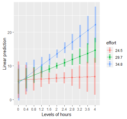
# via {emmeans}
mylist <- list(hours = seq(0,4, by = 0.4), effort = c(eff_low, eff, eff_high))
emmip(contcont, effort ~ hours, at = mylist, CIs = TRUE)

# via {marginaleffects}
plot_predictions(contcont, condition = c("hours", "effort")) # creates it's own subset of values for effort
Predicted Outcome vs IV (newdata) by Moderator (new data)
- For each value of effort, the slope of the hours line at the mean of hours (for that effort level) is the value of the hours marginal effect
Interpretation:
- Suggests that hours spent exercising is only effective for weight loss if we put in more effort. (i.e. as effort increases so does the effect of hours)
- At the highest levels of effort, we achieve higher weight loss for a given time input.
ggplot
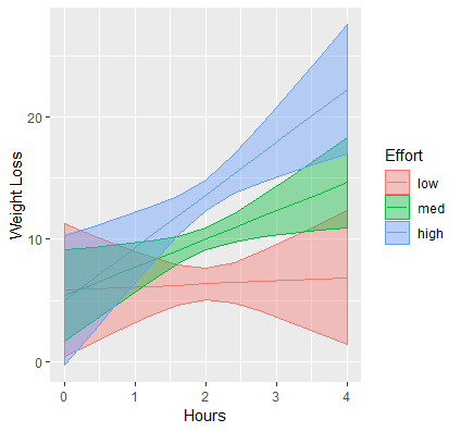
# via {emmeans}
contcontdat <- emmip(contcont,effort~hours,at=mylist, CIs=TRUE, plotit=FALSE)
contcontdat$feffort <- factor(contcontdat$effort)
levels(contcontdat$feffort) <- c("low","med","high")
ggplot(data=contcontdat, aes(x=hours,y=yvar, color=feffort)) +
    geom_line() +
    geom_ribbon(aes(ymax=UCL, ymin=LCL, fill=feffort), alpha=0.4) +
    labs(x="Hours", y="Weight Loss", color="Effort", fill="Effort")

# via {marginaleffects}
moose <- predictions(contcont, newdata = datagrid(hours = seq(0,4, by = 0.4),
                                                  effort = c(eff_low, eff, eff_high),
                                                  grid.type = "counterfactual"))
ggplot(data=moose, aes(x=hours,y=predicted, color=factor(effort))) +
  geom_line() +
  geom_ribbon(aes(ymax=conf.high, ymin=conf.low, fill=factor(effort)), alpha=0.4) +
  labs(x="Hours", y="Weight Loss", color="Effort", fill="Effort")
Test pairwise differences (contrasts) of marginal effects
emtrends(contcont, pairwise ~effort, var="hours",at=mylist) #> $contrasts #> contrast estimate SE df t.ratio p.value #> 24.5 - 29.7 -2.05 0.975 896 -2.098 0.0362 #> 24.5 - 34.8 -4.05 1.931 896 -2.098 0.0362 #> 29.7 - 34.8 -2.01 0.956 896 -2.098 0.0362 #> Results are averaged over the levels of: hours- {marginaleffects} doesn’t do this from what I can tell and IMO looking at contrasts of simple effects (next section) is a better method
- {emmeans}
- pairwise ~effort tells the function that we want pairwise differences of the marginal effects of var=“hours” for each level of effort specified “at=mylist”
- hours not specified in mylist just the 3 values for effort
- The results are with the arg, adjust=“none”, which removes the Tukey multiple test adjustment. Removed it from the code, because it’s bad practice.
- pairwise ~effort tells the function that we want pairwise differences of the marginal effects of var=“hours” for each level of effort specified “at=mylist”
- Interpretation
- A one unit change in hours when effort is high (34.8) results is 4 lbs more weight loss than a one unit change in hours when effort is low (24.5)
- Based on the NHST, all the marginal effects are significantly different from each other
- For continuous:continuous, p-values will all be the same and identical the interaction p-value of the model (has to do with the slope formula)
- Testing the simple effects contrasts (see below) may be the better option
Test pairwise differences (contrasts) of Simple Slopes
# via {emmeans} mylist <- list(hours = 4, effort = c(eff_low, eff_high)) emmeans(contcont, pairwise ~ hours*effort, at=mylist) #> $emmeans #> hours effort emmean SE df lower.CL upper.CL #> 4 24.5 6.88 2.79 896 1.4 12.4 #> 4 34.8 22.26 2.68 896 17.0 27.5 #> Confidence level used: 0.95 #> $contrasts #> contrast estimate SE df t.ratio p.value #> 4,24.5 - 4,34.8 -15.4 3.97 896 -3.871 0.0001 # via {marginaleffects} comparisons(contcont, variables = list(effort = c(eff_low, eff_high)), newdata = datagrid(hours = 4)) |> tidy() #> rowid type term contrast_effort comparison std.error statistic p.value conf.low conf.high effort hours #> 1 1 response interaction 34.8 - 24.5 15.37904 3.97295 3.870938 0.0001084175 7.592203 23.16588 29.65922 4 # alternate (difference in results could be due to rounding of eff_low, eff_high) comparisons(contcont, variables = list(effort = "2sd"), newdata = datagrid(hours = 4, grid.type = "counterfactual")) |> tidy() #> type term contrast_effort estimate std.error statistic p.value conf.low conf.high #> 1 response interaction (x + sd) - (x - sd) 15.35743 3.967367 3.870938 0.0001084175 7.581535 23.13333- One reason to look at the tests for the predicted means contrast instead of the slope contrasts is the constant p-value across slope contrasts (see above)
- If hours isn’t specified
emmeansholds hours at the sample mean.- Using {marginaleffects} and holding hours at sample mean (and probably every other variable in the model),
comparisons(contcont, variables = list(effort = "2sd")) |> tidy()
- Using {marginaleffects} and holding hours at sample mean (and probably every other variable in the model),
- Specification
- hours has a fixed value and the moderator is allowed to vary between high and low effort
- emmeans
- pairwise ~ hours*effort to tell the function that we want pairwise contrasts of each distinct combination of [hours{.var-text} and effort specified at=mylist
- marginaleffects
- effort = “2d” says compare (effort + 1 sd) to (effort - 1 sd)
- grid.type = “counterfactual” because there is no observation in the data with hours = 4
- Interpretation
- Based on the NHST, the difference between the predicted means of high and low effort are significantly different from each other when hours = 4
- After 4 hours of exercise, high effort (34.8) will result in about 15 pounds more weight loss than low effort (24.5) on average.
Continuous:Binary
The change in the slope of the continuous (IV) after a change from the reference level to the other level in the binary (Moderator)
- Note that this value is an additional change to the effect of the continuous (i.e when binary = 1, the effect = continuous effect + interaction effect)
Significant means that the factor variable does increase/decrease the effect of the continuous variable
Example: Does the effect of workout duration in hours (IV) on weight loss (Outcome) change because you are a male or female (Moderator)?
dat <- dat |>
  mutate(gender = factor(gender, labels = c("male", "female")) # male = 1, female = 2,
        gender = relevel(gender, ref = "female")
  )
contcat <- lm(loss ~ hours * gender, data=dat)
#>                  Estimate Std. Error t value Pr(>|t|)
#> (Intercept)         3.335      2.731   1.221    0.222
#> hours               3.315      1.332   2.489    0.013 *
#> gendermale          3.571      3.915   0.912    0.362
#> hours:gendermale   -1.724      1.898  -0.908    0.364
Intercept (\(\beta_0\)): Predicted weight loss when Hours = 0 in the reference group of Gender, which is females.
hours (\(\beta_1\), Independent Variable): The marginal effect of hours for the reference group (e.g. females).
- hours marginal effect for males is \(\beta_1 + \beta_3\) or
emtrends(contcat, ~ gender, var="hours")will give both marginal effects
- hours marginal effect for males is \(\beta_1 + \beta_3\) or
gendermale (\(\beta_2\), Moderator) (reference group: female): The difference in the effect of being male compared to female at hours = 0.
hours:gendermale (\(\beta_3\)): The difference in the marginal effects of hours for males to hours for females.
emtrendscan also give thesummarystats for the interaction (sign different in this case, since difference is from the reference group, female)hours_slope <- emtrends(contcat, pairwise ~ gender, var="hours") hours_slope$contrasts #> contrast estimate SE df t.ratio p.value #> female - male 1.72 1.9 896 0.908 0.3639
Marginal effects of continuous (IV) by each level of the categorical (moderator)
# via {emmeans} emtrends(contcat, ~ gender, var="hours") #> gender hours.trend SE df lower.CL upper.CL #> female 3.32 1.33 896 0.702 5.93 #> male 1.59 1.35 896 -1.063 4.25 # via {marginaleffects} slopes(contcat) |> tidy(by = "gender") #> type term contrast gender estimate std.error statistic p.value conf.low conf.high #> 1 response hours dY/dX male 1.59113665 1.3523002 1.1766150 0.23934921 -1.0593230 4.241596 #> 2 response hours dY/dX female 3.31506746 1.3316491 2.4894453 0.01279426 0.7050833 5.925052 #> 3 response gender male - female male 0.09616813 0.9382760 0.1024945 0.91836418 -1.7428191 1.935155 #> 4 response gender male - female female 0.14194405 0.9382968 0.1512784 0.87975610 -1.6970840 1.980972- {emmeans}
- ~gender says obtain separate estimates for females and males
- var=“hours” says obtain marginal effects (or trends) for hours
- {marginaleffects}
- Can also use
summary(by = "gender")
- Can also use
- Interpretation
- hours by female is the same as the model coefficient above.
- See model interpretation above
- hours by female is the same as the model coefficient above.
- {emmeans}
Simple effects at values of the moderator
# via {emmeans} mylist <- list(hours=c(0,2,4),gender=c("male","female")) emcontcat <- emmeans(contcat, ~ hours*gender, at=mylist) contrast(emcontcat, "pairwise",by="hours") #> hours = 0: #> contrast estimate SE df t.ratio p.value #> male - female 3.571 3.915 896 0.912 0.3619 #> hours = 2: #> contrast estimate SE df t.ratio p.value #> male - female 0.123 0.938 896 0.131 0.8955 #> hours = 4: #> contrast estimate SE df t.ratio p.value #> male - female -3.325 3.905 896 -0.851 0.3948 # via {marginaleffects} comparisons(contcat, variables = "gender", newdata = datagrid(hours = c(0, 2, 4))) #> rowid type term contrast_gender comparison std.error statistic p.value conf.low conf.high gender hours #> 1 1 response interaction male - female 3.5710607 3.914762 0.9122038 0.3616614 -4.101731 11.243853 male 0 #> 2 2 response interaction male - female 0.1231991 0.937961 0.1313478 0.8955002 -1.715171 1.961569 male 2 #> 3 3 response interaction male - female -3.3246625 3.905153 -0.8513527 0.3945735 -10.978622 4.329297 male 4- The moderator is now hours
- Note that output for hours = 0, the effect 3.571 matches the \(\beta_2\) coefficient
- Interpretation
- As hours increases, the male versus female difference becomes more negative (females are losing more weight than males)
Plotting the continuous by binary interaction
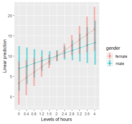
# via {emmeans} mylist <- list(hours=seq(0,4,by=0.4),gender=c("female","male")) emmip(contcat, gender ~hours, at=mylist,CIs=TRUE)- For ggplot, see continuous:continuous >> Plot marginal effects for IV section (Should be similar code)
- Interpretation
- Although it looks like there’s a cross-over interaction, the large overlap in confidence intervals suggests that the slope of hours is not different between males and females
- Confirmed by looking at the standard error of the interaction coefficient (1.898) is large relative to the absolute value of the coefficient itself (1.724)
- Although it looks like there’s a cross-over interaction, the large overlap in confidence intervals suggests that the slope of hours is not different between males and females
Categorical:Categorical
From {marginaleffects} Contrasts vignette, “Since derivatives are only properly defined for continuous variables, we cannot use them to interpret the effects of changes in categorical variables. For this, we turn to contrasts between adjusted predictions (aka Simple Effects).”
- i.e. Contrasts of marginal effects aren’t possible
2x3 cat:cat interaction
Example: Do males and females (IV) lose weight (Outcome) differently depending on the type of exercise (Moderator) they engage in?
dat <- dat |>
  mutate(gender = factor(gender, labels = c("male", "female")),
        gender = relevel(gender, ref = "female"),
        prog = factor(prog, labels = c("jog","swim","read")),
        prog = relevel(prog, ref="read")
  )
catcat <- lm(loss ~ gender * prog, data = dat)
#>                     Estimate Std. Error t value Pr(>|t|)
#> (Intercept)          -3.6201     0.5322  -6.802 1.89e-11 ***
#> gendermale           -0.3355     0.7527  -0.446    0.656
#> progjog               7.9088     0.7527  10.507  < 2e-16 ***
#> progswim             32.7378     0.7527  43.494  < 2e-16 ***
#> gendermale:progjog    7.8188     1.0645   7.345 4.63e-13 ***
#> gendermale:progswim  -6.2599     1.0645  -5.881 5.77e-09 ***
Description
- Intercept (\(\beta_0\)): The intercept, or the predicted weight loss when gendermale = 0, progjog = 0, and progswim = 0
- i.e. The intercept for females in the reading program
- gendermale (\(\beta_1\)): The simple effect of males when progjog = 0 and progswim = 0
- i.e. The male – female weight loss in the reading group
- progjog (\(\beta_2\)): the simple effect of jogging when gendermale = 0
- i.e. The difference in weight loss between jogging versus reading for females
- progswim (\(\beta_3\)): The simple effect of swimming when gendermale = 0
- i.e. The difference in weight loss between swimming versus reading for females
- gendermale:progjog (\(\beta_4\)): The male effect (male – female) in the jogging condition versus the male effect in the reading condition.
- Also, the jogging effect (jogging – reading) for males versus the jogging effect for females.
- gendermale:progswim (\(\beta_5\)): the male effect (male – female) in the swimming condition versus the male effect in the reading condition.
- Also, the swimming effect (swimming – reading) for males versus the swimming effect for females.
- gender is the independent variable
- Prog is the moderator
- Reference Groups
- prog == read
- gender == female
- \(\beta_1 + \beta_4\): The marginal effect of gender == males in the prog == jogging group.
- \(\beta_1 + \beta_5\): The marginal effect of gender == males in the prog == swimming group.
- Intercept (\(\beta_0\)): The intercept, or the predicted weight loss when gendermale = 0, progjog = 0, and progswim = 0
Marginal Means for all combinations of the interaction variable levels
# via {emmeans} emcatcat <- emmeans(catcat, ~ gender*prog) #> gender prog emmean SE df lower.CL upper.CL #> female read -3.62 0.532 894 -4.66 -2.58 #> male read -3.96 0.532 894 -5.00 -2.91 #> female jog 4.29 0.532 894 3.24 5.33 #> male jog 11.77 0.532 894 10.73 12.82 #> female swim 29.12 0.532 894 28.07 30.16 #> male swim 22.52 0.532 894 21.48 23.57 # via {marginaleffects} predictions(catcat, variables = c("gender", "prog")) #> rowid type predicted std.error conf.low conf.high gender prog #> 1 1 response 11.772028 0.5322428 10.727437 12.816619 male jog #> 2 2 response 22.522383 0.5322428 21.477792 23.566974 male swim #> 3 3 response -3.955606 0.5322428 -5.000197 -2.911016 male read #> 4 4 response 4.288681 0.5322428 3.244091 5.333272 female jog #> 5 5 response 29.117691 0.5322428 28.073100 30.162282 female swim #> 6 6 response -3.620149 0.5322428 -4.664740 -2.575559 female read- Marginal means generated using the regression coefficients
.png)
- Kinda weird. Since these are predicted means (i.e. outcome values), I wouldn’t have thought they could be generated by the model coefficients. ¯\_(ツ)_/¯
- Interpretation
- females in the reading program have an estimated weight gain of 3.62 pounds
- males in the swimming program have an average weight loss of 22.52 pounds
- Marginal means generated using the regression coefficients
Simple Effects of the IV for all values of the moderator variable
# via {emmeans} contrast(emcatcat, "revpairwise", by="prog") # see above code chunk for emcatcat #> prog = read: #> contrast estimate SE df t.ratio p.value #> male - female -0.335 0.753 894 -0.446 0.6559 #> prog = jog: #> contrast estimate SE df t.ratio p.value #> male - female 7.483 0.753 894 9.942 <.0001 #> prog = swim: #> contrast estimate SE df t.ratio p.value #> male - female -6.595 0.753 894 -8.762 <.0001 # via {marginaleffects} comparisons(catcat, variables = "gender", newdata = datagrid(prog = c("read", "jog", "swim"))) #> rowid type term contrast_gender comparison std.error statistic p.value conf.low conf.high gender prog #> 1 1 response interaction male - female -0.3354569 0.7527049 -0.4456686 6.558367e-01 -1.810731 1.139818 male read #> 2 2 response interaction male - female 7.4833463 0.7527049 9.9419388 2.734522e-23 6.008072 8.958621 male jog #> 3 3 response interaction male - female -6.5953078 0.7527049 -8.7621425 1.915739e-18 -8.070582 -5.120033 male swim- {emmeans}
- revpairwise rather than pairwise because by default the reference group (female) would come first
- The results are with the arg, adjust=“none”, which removes the Tukey multiple test adjustment. Removed it from the code, because it’s bad practice.
- Interpretation
- male effect for jogging and swimming are significant at the 0.05 level (with no adjustment of p-values), but not for the reading condition.
- males lose more weight in the jogging condition (positive) but females lose more weight in the swimming condition (negative)
- {emmeans}
Plotting the categorical by categorical interaction
{emmeans}
emmip(catcat, prog ~ gender,CIs=TRUE)
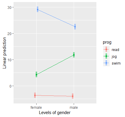
{ggplot2}
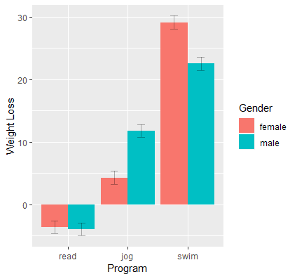
catcatdat <- emmip(catcat, gender ~ prog, CIs=TRUE, plotit=FALSE) #> gender prog yvar SE df LCL UCL tvar xvar #> 1 female read -3.620149 0.5322428 894 -4.664740 -2.575559 female read #> 2 male read -3.955606 0.5322428 894 -5.000197 -2.911016 male read #> 3 female jog 4.288681 0.5322428 894 3.244091 5.333272 female jog #> 4 male jog 11.772028 0.5322428 894 10.727437 12.816619 male jog #> 5 female swim 29.117691 0.5322428 894 28.073100 30.162282 female swim #> 6 male swim 22.522383 0.5322428 894 21.477792 23.566974 male swim # via {marginaleffects} predictions(catcat, variables = c("gender", "prog")) ggplot(data=catcatdat, aes(x=prog,y=yvar, fill=gender)) + geom_bar(stat="identity",position="dodge") + geom_errorbar(position=position_dodge(.9),width=.25, aes(ymax=UCL, ymin=LCL),alpha=0.3) labs(x="Program", y="Weight Loss", fill="Gender")- I think I like the emmeans plot better
- Values come from the Marginal Means for all combinations of the interaction variable levels section above
Logistic Regression
Misc
- * categorical:categorical and continuous:continuous should be should be similar to analysis for binary:continuous and the code/analysis in the OLS section *
- For more details on these other interaction types see the article linked below
- Misc
- Notes from
- How Can I Understand A Categorical By Continuous Interaction In Logistic Regression
- Deciphering Interactions In Logistic Regression
- See this article for continuous:continuous, cat:cat
- Also see
- Reminder: OR significance is being different from 1 and log odds ratios (logits) significance is being different from 0
- Although the interaction is quantified appropriately by the interaction coefficient when interpreting effects on the scale of log-odds or log-counts, the interaction effect will not reduce to the coefficient of the the interaction coefficient when describing effects on the natural response scale (i.e. probabilities, counts) because of the inverse-link transformation.
- In order to get e.g. probabilities, the inverse-link function must be used, and this complicates the derivatives of the marginal effect calculation. The chain rule must be appied. This means the interaction effect is no longer equivalent to the interaction coefficient.
- Therefore, effects or contrasts are differences in marginal effects rather than coefficients
- Interaction effects represent change in a marginal effect of one predictor for a change in another predictoreraction effects represent change in a marg
- Standard errors of point estimate values of interaction effects (as well as their corresponding statistical significance) may also vary as a function of the predictors.
- Need to decide whether the interaction is to be conceptualized in terms of log odds (logits) or odds ratios or probability
- An interaction that is significant in log odds may not be significant in terms of probability or vice versa
- Even if they do agree, the p-values do not have the be the same. (See below, binary:continuous >> Simple Effects >> second example >> probabilities)
- An interaction that is significant in log odds may not be significant in terms of probability or vice versa
- Notes from
Continuous:Continuous
Example: Spam or Ham (source)
How do linguistic toxicity patterns (captured by PCA components) interact with message characteristics like length and punctuation to identify spam? And more importantly, how can we interpret these relationships meaningfully?
pacman::p_load( dplyr, brms, marginaleffects, ggdist ) model_data <- model_data |> mutate(across(all_of( c("pc_aggression", "word_count", "pc_incoherence", "exclamation_count")), ~ as.numeric(scale(.x)) ) )- is_spam - Our outcome variable; a binary classification indicating spam or legitimate communication.
- pc_aggression & pc_incoherence - Principal components that were extracted from Google’s Perspective API toxicity scores capturing sophisticated linguistic patterns:
- pc_aggression: threatening, toxic, and insulting language patterns.
- pc_incoherence: inflammatory, incoherent, or unsubstantial messages.
- word_count - The total number of words per message (includes squared term to capture non-linear relationships).
- exclamation_count - The number of exclamation points, a simple but telling spam feature.
- Standardizing the predictors first since our prior will have a mean of 0
1d_expected <- 0.3 prior_sd <- d_expected * pi / sqrt(3) # ≈ 0.54 2priors <- c( prior(normal(0, 0.54), class = b) ) spam_model <- brm( 3 is_spam ~ (pc_aggression + pc_incoherence) * (word_count + exclamation_count), data = model_data, family = bernoulli(), prior = priors, cores = 4, iter = 2000, warmup = 1000, chains = 4, seed = 123 )- 1
- Set our priors based on expected small-to-medium effects
- 2
- Setting class = b says all slopes will have the same prior
- 3
- Formula syntax specifies a specific combination subset of all 2-way interactions
marginal_effects <- avg_slopes(spam_model, type = "response") marginal_effects #> Term Estimate 2.5 % 97.5 % #> exclamation_count 0.0246 0.0104 0.0387 #> pc_aggression -0.0410 -0.0565 -0.0256 #> pc_incoherence -0.1709 -0.1834 -0.1577 #> word_count 0.0803 0.0635 0.0973 #> #> Type: response #> Comparison: dY/dX bayestestR::ci(marginal_effects, method = "HDI") #> Highest Density Interval #> #> term | contrast | 95% HDI #> --------------------------------------------- #> exclamation_count | dY/dX | [ 0.01, 0.04] #> pc_aggression | dY/dX | [-0.06, -0.03] #> pc_incoherence | dY/dX | [-0.18, -0.16] #> word_count | dY/dX | [ 0.06, 0.10]- Computes the average marginal effects which tells us how much each feature changes the probability of spam classification, averaged across all observations
- On average, a 1 sd increase in word_count results in an increase of 0.0803 percentage points of the probability of being spam.
- By default, {marginaleffects} credible intervals in bayesian models are built as equal-tailed intervals (ETI). This can be changed to a highest density interval (HDI) by setting a global option:
options("marginaleffects_posterior_interval" = "eti")options("marginaleffects_posterior_interval" = "hdi")
# Interaction 1 incoherence_by_wordcount <- avg_slopes( spam_model, variables = "pc_incoherence", newdata = datagrid( word_count = quantile(model_data$word_count, probs = c(.05, .25, .50, .75, .95)) ), type = "response" ) #> Estimate 2.5 % 97.5 % #> -0.193 -0.21 -0.175 #> #> Term: pc_incoherence #> Type: response #> Comparison: dY/dX # Interaction 2 incoherence_by_exclamation <- avg_slopes( spam_model, variables = "pc_incoherence", newdata = datagrid( exclamation_count = quantile(model_data$exclamation_count, probs = c(.05, .25, .50, .75, .95)) ), type = "response" ) # Interaction 3 aggression_by_exclamation <- avg_slopes( spam_model, variables = "pc_aggression", newdata = datagrid( exclamation_count = quantile(model_data$exclamation_count, probs = c(.05, .25, .50, .75, .95)) ), type = "response" ) # Interaction 4 aggression_by_wordcount <- avg_slopes( spam_model, variables = "pc_aggression", newdata = datagrid( word_count = quantile(model_data$word_count, probs = c(.05, .25, .50, .75, .95)) ), type = "response" )- type = “response”- Computes posterior draws of the expected value using the
brms::posterior_epredfunction- Outputs a distribution of means which shows the amount of uncertainty around the mean
- The first interaction is an estimate of how incoherence’s effect changes with word count. The slope of incoherence is averaged across the specified quantiles of wordcount.
- On average, the probability of spam decreases by 0.193 percentage points when incoherence increases by 1 standard deviation (standardized predictors) after taking word count into account.
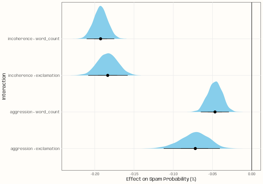
# Extract draws as rvars for each interaction draws_df <- bind_rows( get_draws(incoherence_by_wordcount, shape = "rvar") |> as.data.frame() |> mutate(interaction = "incoherence × word_count"), get_draws(incoherence_by_exclamation, shape = "rvar") |> as.data.frame() |> mutate(interaction = "incoherence × exclamation"), get_draws(aggression_by_exclamation, shape = "rvar") |> as.data.frame() |> mutate(interaction = "aggression × exclamation"), get_draws(aggression_by_wordcount, shape = "rvar") |> as.data.frame() |> mutate(interaction = "aggression × word_count") ) draws_df |> ggplot(aes(y = interaction, xdist = rvar)) + stat_slabinterval( colour = "black", linewidth = .5, fill = "skyblue" ) + labs(x = "Effect on Spam Probability (%)", y = "Interaction") + geom_vline(xintercept = 0, colour = "black", linewidth = .5) + theme_notebook()- rvar is a random variable datatype. (See Bayes, Inference >> Misc)
- Basicially just an array datatype that is built to work with other packages.
- Distribution of means for each interaction is visualized. The point of the interval for each distribution shows the median by default.
Binary:Continuous
- Example:
Description
dat_clean <- dat |> mutate(f = factor(f, labels = c("female", "male"))) concat <- glm(y ~ f*s, family = binomial, data = dat_clean) summary(concat) #> Estimate Std. Error z value Pr(>|z|) #> (Intercept) -9.25380 1.94189 -4.765 1.89e-06 *** #> fmale 5.78681 2.30252 2.513 0.0120 * #> s 0.17734 0.03644 4.867 1.13e-06 *** #> fmale:s -0.08955 0.04392 -2.039 0.0414 *- y: Binary Outcome
- s (IV): Continuous Variable
- f (moderator): Gender variable with female as the reference
- cv1: Continuous Adjustment Variable
Marginal effects of continuous (IV) by each level of the categorical (moderator)
# via {marginaleffects} slopes(concat, variables = "s") |> tidy(by = "f") #> type term f estimate std.error statistic p.value conf.low conf.high #> 1 response s male 0.01473352 0.003237072 4.551498 5.32654e-06 0.00838898 0.02107807 #> 2 response s female 0.02569069 0.001750066 14.679842 0.00000e+00 0.02226062 0.02912075- Interpetation
- Increasing s by 1 unit given that the person is male will result in around a 1% increase on average in the probability of the event, y.
- Interpetation
Simple effects at values of the IV
# via {marginaleffects} comp <- comparisons(concat2, variables = "f", newdata = datagrid(s = seq(20, 70, by = 2))) head(comp) #> rowid type term contrast_f comparison std.error statistic p.value conf.low conf.high f s #> 1 1 response interaction male - female 0.1496878 0.09871431 1.516374 0.12942480 -0.043788674 0.3431643 male 20 #> 2 2 response interaction male - female 0.1724472 0.10430544 1.653291 0.09827172 -0.031987695 0.3768821 male 22 #> 3 3 response interaction male - female 0.1975119 0.10886095 1.814351 0.06962377 -0.015851616 0.4108755 male 24 #> 4 4 response interaction male - female 0.2246979 0.11209440 2.004542 0.04501204 0.004996938 0.4443989 male 26 #> 5 5 response interaction male - female 0.2536377 0.11376972 2.229395 0.02578761 0.030653136 0.4766222 male 28 #> 6 6 response interaction male - female 0.2837288 0.11375073 2.494303 0.01262048 0.060781436 0.5066761 male 30- Shows the predicted value contrasts for the moderator at different values of the independent variable.
- concat2 model defined in “Simple Effects at values of the moderator and adjustment variable” (see below)
- For
comparisons, the default is type = “response” so the output is probabilities. (type = “link” for log-ORs aka logits) - Interpretation
- For s = 26, 28, and 30, there is substantial evidence that there are differences in male and female probabilites of the event, y.
- Example: (article)
- Description
- lowbwt: Binary Outcome, low birthweight = 1
- age (IV): Continuous, Age of the mother
- ftv (moderator): Binary, whether or not the mother made frequent physician visits during the first trimester of pregnancy
- Simple Effects: Odds Ratios
.png)
- ORftv is the odds-ratio contrast of (ftv = 1) - (ftv = 0) at the specified age of the mother
- Interpretation
- A mother at the age of 30 who visits the physician frequently has 0.174 times the odds of having a low birth weight baby as compared to those of the same age who don’t visit the doctor frequently
- For women whose ages are between 17 and 24, the 95% confidence intervals of the odds ratios include the null value of 1, so we do not have strong evidence of an association between frequent doctor visits and low birth weight for that age range.
- For mothers aged 25 years and older, the odds of having a low birth weight baby significantly decrease if the mother frequently visits her physician.
- Simple Effects: Probabilities
.png)
- “Difference in probability” is the probability contrast of (ftv = 1) - (ftv = 0) at the specified age of the mother
- Note that the results agree with the OR results, but the pvals are different
- So it’s probably possible that in terms of “significance,” you could get different conclusions based on the metric used.
- Interpretation
- For young mothers (less than 24 years old), we do not have strong evidence of an association between low birth weight and frequent physician [visits]{.var-text.
- For mothers aged 25 years and older, we reject the null hypothesis of no difference in probability between those with frequent physician visits and those without.
- Overall, the difference between the probability of low birth weight comparing those with frequent visits to those without increases as the mother’s age increases.
- Description
- Shows the predicted value contrasts for the moderator at different values of the independent variable.
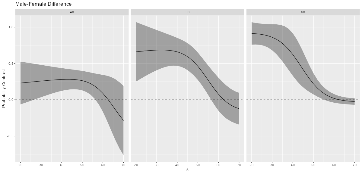
Plot the simple effects
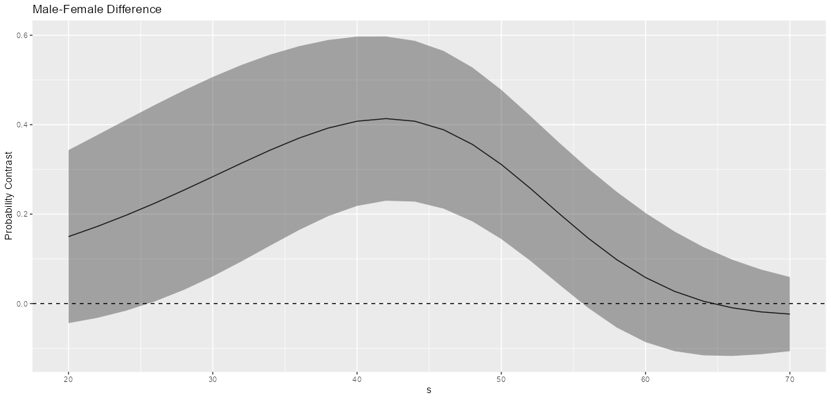
ggplot(comp, aes(x = s, y = comparison)) + geom_line() + geom_ribbon(aes(ymax=conf.high, ymin=conf.low), alpha=0.4) + geom_hline(yintercept=0, linetype="dashed") + labs(title = "Male-Female Difference", y="Probability Contrast")- {marginaleffects}
- You change the
comparisons(see above) type arg to type = link to get log-ORs (aka logits) instead of probabilities and then plot
- You change the
- Interpretation
- The difference in probabilities for male and females is statistically significant between values of s approximately between 28 to 55.
- {marginaleffects}
Simple Effects at values of the moderator and adjustment variable
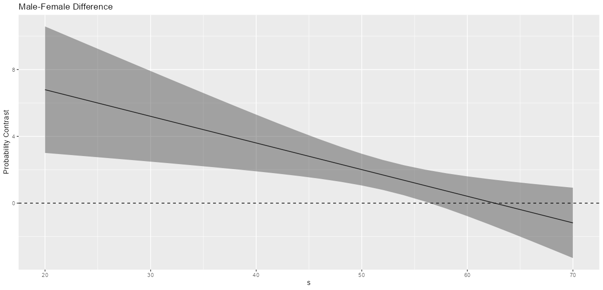
concat2 <- glm(y ~ f*s + cv1, family = binomial, data = dat_clean)
comp2 <- comparisons(concat2,
                    variables = "f",
                    newdata = datagrid(s = seq(20, 70, by = 2),
                                      cv1 = c(40, 50, 60)))
head(comp2)
#>   rowid    type        term    contrast_f comparison  std.error statistic      p.value    conf.low conf.high    f  s cv1
#> 1    1 response interaction male - female  0.2307214 0.15001700  1.537968 1.240564e-01 -0.06330656 0.5247493 male 20  40
#> 2    2 response interaction male - female  0.6603841 0.20879886  3.162777 1.562722e-03  0.25114590 1.0696224 male 20  50
#> 3    3 response interaction male - female  0.9135206 0.07865839 11.613773 3.507873e-31  0.75935304 1.0676882 male 20  60
#> 4    4 response interaction male - female  0.2361502 0.14294726  1.652009 9.853270e-02 -0.04402131 0.5163217 male 22  40
#> 5    5 response interaction male - female  0.6663811 0.19447902  3.426494 6.114278e-04  0.28520927 1.0475530 male 22  50
#> 6    6 response interaction male - female  0.9097497 0.07571970 12.014703 2.974362e-33  0.76134178 1.0581575 male 22  60
Plot simple effects and facet by values of the adjustment variable
ggplot(comp2, aes(x = s, y = comparison, group = factor(cv1))) + geom_line() + geom_ribbon(aes(ymax=conf.high, ymin=conf.low), alpha=0.4) + geom_hline(yintercept=0, linetype="dashed") + facet_wrap(~ cv1) + labs(title = "Male-Female Difference", y="Probability Contrast")- Interpretation
- It seems clear from looking at the three graphs that the male-female difference in probability increases as cv1 increases except for high values of s.
- Interpretation
Poisson/Neg.Binomial
- Misc
- Notes from Paper Interpreting interaction effects in generalized linear models of nonlinear probabilities and counts
- Although the interaction is quantified appropriately by the interaction coefficient when interpreting effects on the scale of log-odds or log-counts, the interaction effect will not reduce to the coefficient of the the interaction coefficient when describing effects on the natural response scale (i.e. probabilities, counts) because of the inverse-link transformation.
- In order to get e.g. probabilities, the inverse-link function must be used, and this complicates the derivatives of the marginal effect calculation. The chain rule must be appied. This means the interaction effect is no longer equivalent to the interaction coefficient.
- Therefore, effects or contrasts are differences in marginal effects rather than coefficients
- Interaction effects represent change in a marginal effect of one predictor for a change in another predictoreraction effects represent change in a marg
- Standard errors of point estimate values of interaction effects (as well as their corresponding statistical significance) may also vary as a function of the predictors.
- Types
- Continuous:Continuous: The rate-of-change in the marginal effect of one predictor given a change in another predictor
- Also, the amount the effect of \(x_1\) on \(\mathbb{E}[Y\;|\;x]\) changes for every one-unit increase in \(x_2\) (and vice versa), holding all else constant.
- Continuous:Discrete: The Difference in the marginal effect of the continuous predictor between two selected values of the discrete predictor
- Example: Poisson outcome (population)
.png)
- \(x_1\) is continuous, \(x_2\) is continuous, \(x_3\) is binary (e.g. sex where female = 1).
- The interaction effect, \(\gamma^2_{13}\), of \(x_1x_3\) is the difference between the marginal effect of \(x_1\) for females versus males
- Note that \(x_2\) is included in the effect calculation for an interaction it isn’t part of
- Specific values for \(x_1\) and \(x_2\) must be chosen to the calculate the value of the effect
.png)
- For \(x_2\), the 25th, 50th, 75th quartiles are used and \(x_1\) would be held at one value of substantive interest (e.g. mean)
- Standard errors via delta method for all 3 values can be computed along with p-values
- Visual
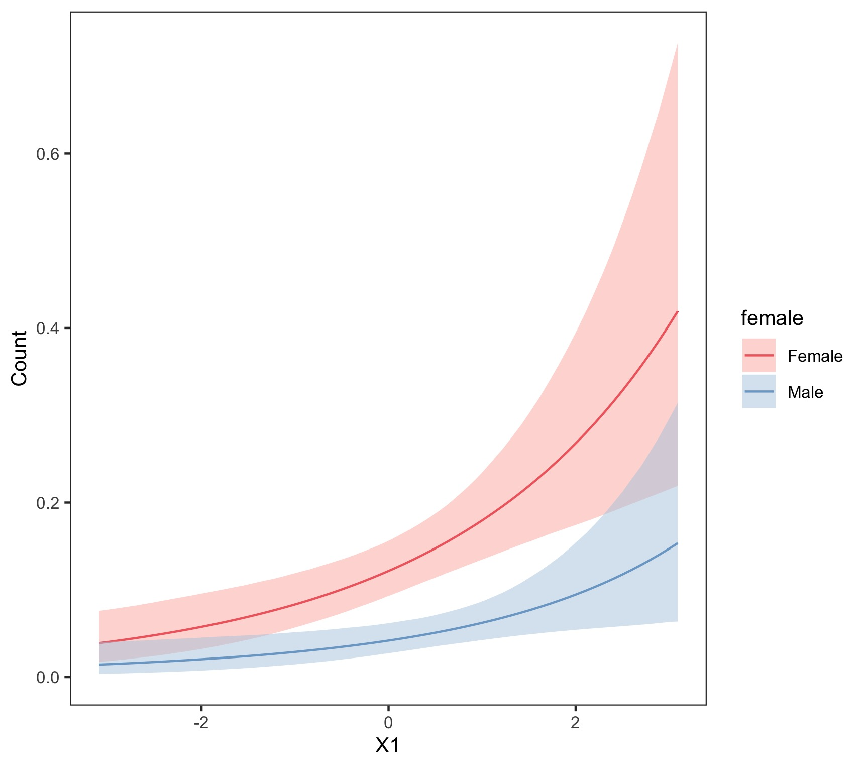
- \(x_2\) is held at its mean, and various values of \(x_1\) are used
- Interpretation: the expected population (count of \(Y\)) is larger among females than males across all values of \(x_1\) with \(x_2\) held at its mean.
- Example: Poisson outcome (population)
- Discrete:Discrete: The difference between the model evaluated at two categories of one variable (a, b) minus the difference in this model evaluated at two categories of another variable (c, d) (aka discrete double difference)
- Continuous:Continuous: The rate-of-change in the marginal effect of one predictor given a change in another predictor