Base R
Misc
Packages
- {poorman} - Dependency free versions of {dplyr} verbs that help you solve the most common data manipulation challenges
Magrittr + base
mtcars %>% {plot(.$hp, .$mpg)} mtcars %$% plot(hp, mpg)- By wrapping the RHS in curly braces, we can override the rule where the LHS is passed to the first argument ## Options {#sec-r-baser-opts .unnumbered}
Remove scientific notation
options(scipen = 999)Wide and long printing tibbles
# in .Rprofile makeActiveBinding(".wide", function() { print(.Last.value, width = Inf) }, .GlobalEnv)- After printing a tibble, if you want to see it in wide, then just type .wide + ENTER.
- Can have similar bindings for `.long` and `.full`.
Heredocs - Powerful feature in various programming languages that allow you to define a block of text within the code, preserving line breaks, indentation, and other whitespace.
text <- r"(
This is a
multiline string
in R)"

cat(text)
Selective function importing (R \(\ge\) 4.0) (source)
library(stringr, include.only = c("str_extract", "str_remove"))Super Assignment (
<<-)- It never creates a variable in the current environment, but instead modifies an existing variable found in a parent environment
- If
<<-doesn’t find an existing variable, it will create one in the global environment. - Most often used in conjunction with a function factory (See Advanced R, Sect. 10.2.4)
Downloading, Reading, and Writing
Set internet timeout value
Environment variable
R_DEFAULT_INTERNET_TIMEOUT=300Options
options(timeout = max(300, getOption("timeout")))
Downloading and reading .rda and .RData via URL
# option 1 pop_url <- url("https://raw.githubusercontent.com/edzer/sdsr/main/data/ch12.rda") load(pop_url) # option 2 url <- "https://raw.githubusercontent.com/edzer/sdsr/main/data/ch12.rda" destfile <- tempfile(fileext = ".rda") download.file(url, destfile, mode = "wb") load(destfile) # option 3 dat_de_pop <- local({ load(url("https://raw.githubusercontent.com/edzer/sdsr/main/data/ch12.rda"), envir = environment()) if (length(ls()) > 1) { mget(ls()) } else { get(ls()[1]) } })loadwill not allow you to assign the loaded object to a name of your choosing, i.e.moose <- load(moose.rda)will not work.localcreates a temporary evaluation environment and ensures no stray variables remain in your workspaceload(..., envir = environment())loads the.rdacontents into the local environment created bylocalls(e)[1]retrieves the (first) object name that was loaded into the local environment.getextracts the actual object from that environment.mgetaccepts a character vector of object names. So, if the .rda file contains multiple objects, this function will load them all in a list.
Download multiple files
urls <-
  c("https://ereporting.blob.core.windows.net/downloadservice/NL_8_28027_2017_timeseries.csv",
    "https://ereporting.blob.core.windows.net/downloadservice/NL_8_28145_2017_timeseries.csv"
)

dest_dir <- "C:/Users/user/Documents/R/Data/no2/raw"
dir.create(dest_dir, recursive = TRUE, showWarnings = FALSE)

dest <- file.path(dest_dir, basename(urls))

# Download with a polite delay between requests
for(i in seq_along(urls)) {
  download.file(urls[i],
                destfile = dest[i],
                mode = "wb") # windows

  # Wait 1-2 seconds between downloads
  if(i < length(urls)) {
    Sys.sleep(1)
  }
}
Reading in zipped files (source)
# unz() lets you read one file from a .zip
one_zipped_csv_among_others <- readr::read_csv(
  unz("lotsa_zipped_csvs.zip", "one_csv.csv")
)

# .zip with a single CSV
one_zipped_csv <- readr::read_csv("big_zipped_file.zip")
User Defined Functions
Anonymous (aka lambda) functions:
\(x) {}(> R 4.1)function(x) { x[which.max(x$mpg), ] } # equivalent to the above \(x) { x[which.max(x$mpg), ] }Define and call an anonymous function at the same time
n <- c(1:10)
moose <- (\(x) x+1)(n)
moose
#> [1]  2  3  4  5  6  7  8  9 10 11
Dots (…)
Misc
- Packages
- {ellipsis}: Functions for testing functions with dots so they fail loudly
- Resources
- Video: Demystifying . . . (dots): R package dev fundamentals (Parry)
- Advanced R, Ch 6.6
- {rlang} dynamic dots: article
- Splice arguments saved in a list with the splice operator,
!!!. - Inject names with glue syntax on the left-hand side of
:=.
- Splice arguments saved in a list with the splice operator,
- Packages
Basic Usage
my_data_frame <- function(...) {
  dots <- list(...)
  dots_names <- names(dots)

  if (is.null(dots_names) || "" %in% dots_names) {
    stop("all arguments must be named")
  }

  list2DF(dots)
}
# errors b/c args not named
my_data_frame(1:10, letters[1:10])
# works
data_frame(id = 1:10, alphabet = letters[1:10])
Some forms I’ve used inside UDFs
1dots <- list(...) init_boot_args <- list(data = dynGet("data"), stat_fun = cles_boot, # internal function group_variables = group_variables, paired = paired) get_boot_args <- append(init_boot_args, dots) 2grp_tbl <- .tbl %>% dplyr::group_by(...) 3.data |> dplyr::reframe({{ array_name }} := purrr::pmap(list(!!!dots), ~list(...)), .by = {{ .grp_var }})- 1
- From {ebtools::get_boot_ci}
- 2
- From {ebtools::add_mase_scale_feat}
- 3
- From {ebtools::to_json_array}
Some tests I used
moose <- function(...) {
  dots <- list(...)
  dots_names <- names(dots)
  if (is.null(dots_names) || "" %in% dots_names {
    stop("All arguments must be named")
  }


  dots <- rlang::enquos(..., .named = TRUE)
  # group column(s) required
  chk::chk_not_empty(dots, x_name = "... (group columns)")


  accepted_styles <- c("W", "B", "C", "S", "U", "minmax", "raw")
  dots <- list(...)
  # Check if "style" is provided in ... and validate
  if ("style" %in% names(dots)) {
    chk::chk_subset(dots$style,
                    accepted_styles,
                    x_name = "style")
  }
}
Nested Functions
f02 <- function(...){
  vv <- list(...)
  print(vv)
}
f01 <- function(...){
  f02(b = 2,...)
}

f01(a=1,c=3)
#> $b
#> [1] 2
#>
#> $a
#> [1] 1
#>
#> $c
#> [1] 3
Subset dots values
add2 <- function(...) {
  ..1 + ..2
}
add2(3, 0.14)
# 3.14
Subset dots dynamically:
...elt(n)- Assign a value to n and get back the value of that argument
- A programmatic way to subset instead of the hard coding way (i.e.
..1)
Number of arguments in … :
...length()
Functions
aggregateaggregate(x, by, FUN)- Can also take a formula,
x ~ group - drop = TRUE means that any groups with zero count are removed.
- na.action controls the treatment of missing values within the data.
- Can also take a formula,
Mean for combinations of two groups
aggregate(df$points, by=list(df$team, df$position), FUN=mean)

#>   Group.1 Group.2    x
#> 1       A       F 86.0
#> 2       B       F 97.0
#> 3       A       G 94.5
#> 4       B       G 88.0
Count distinct values per group (source)
data("mtcars") group_counts <- aggregate( data = mtcars, carb ~ cyl, FUN = function(x) length(unique(x)) ) group_counts #> cyl carb #> 1 4 2 #> 2 6 3 #> 3 8 4- cyl and carb are discrete
- Groups by the cyl variable and applies the
lengthanduniqueto count the number of distinct carb per cyl group
Adding function arguments
dat <- aggregate(tserie ~ month(index(tserie)),
                 FUN = quantile,
                 probs = c(0.05, 0.95))
colnames(dat)[1] <- "Month"
dat
#>  Month    V1.5%      V2.95%
#>    1   -1.7041221   1.2301178
#>    2   -0.9388331   1.7888182
#>    3   -1.3886001   1.5261942
#>    4   -1.0834517   1.5697239
#>    5   -1.6527890   1.0883061
#>    6   -1.4064641   2.1472166
Sum of multiple variables for combinations of groups (source)
exposures <- aggregate(x = assets[c("counterparty.a",
                                    "counterparty.b",
                                    "counterparty.c")],
                       by = assets[c("asset.class", "rating")],
                       FUN = function(market.values){
                               sum(pmax(market.values, 0))
                             })
exposures
#>   asset.class rating counterparty.a counterparty.b counterparty.c
#> 1        bond      A      1.0038714      0.6382029      2.2822936
#> 2      equity      A      0.9841620      1.5178126      0.7745532
#> 3        bond    AAA      0.0000000      0.0000000      0.0000000
#> 4      equity    AAA      0.9026004      0.6029417      0.8629453
aveSort of
group_by+mutate(source)x <- c(1, 2, 3, 1, 2, 3, 3, 3) y <- c(1, 1, 1, 1, 2, 2, 2, 2) # ~~~~~~~~~~~~~~~~~~~~~~~~~~~~~~~~~~~~~~~~~~~~~~~~~~~~~~~~~~~~~ # 1. Sum over `x` using `y` as a 'grouping' variable # ~~~~~~~~~~~~~~~~~~~~~~~~~~~~~~~~~~~~~~~~~~~~~~~~~~~~~~~~~~~~~ ave(x, y, FUN = sum) #> [1] 7 7 7 7 11 11 11 11 # ~~~~~~~~~~~~~~~~~~~~~~~~~~~~~~~~~~~~~~~~~~~~~~~~~~~~~~~~~~~~~ # 2. Number of distinct elements in each group # ~~~~~~~~~~~~~~~~~~~~~~~~~~~~~~~~~~~~~~~~~~~~~~~~~~~~~~~~~~~~~ ave(x, y, FUN = dplyr::n_distinct) #> [1] 3 3 3 3 2 2 2 2 # ~~~~~~~~~~~~~~~~~~~~~~~~~~~~~~~~~~~~~~~~~~~~~~~~~~~~~~~~~~~~~ # 3. Number of times each element of `x` appears # ~~~~~~~~~~~~~~~~~~~~~~~~~~~~~~~~~~~~~~~~~~~~~~~~~~~~~~~~~~~~~ ave(x, x, FUN = length) #> [1] 2 2 4 2 2 4 4 4 # ~~~~~~~~~~~~~~~~~~~~~~~~~~~~~~~~~~~~~~~~~~~~~~~~~~~~~~~~~~~~~ # 4. Indicating how many times each element has occurred so far # ~~~~~~~~~~~~~~~~~~~~~~~~~~~~~~~~~~~~~~~~~~~~~~~~~~~~~~~~~~~~~ x <- c("a", "a", "b", "a", "b", "c") paste0(x, ave(x, x, FUN = seq_along)) #> [1] "a1" "a2" "b1" "a3" "b2" "c1"- Group by “1” and sum. So all the x values that have the same index as y = 1 sum to: 7 = 1 + 2 + 3 + 1. For each y = 1, that calculation is made, so there are 4 sevens.
- Group by “1” and find the number of distinct values. There are 3 distinct values of x when y = 1: 1, 2, and 3.
- x is used for each input. It counts how many times the value appears in the vector. 1 occurs twice, 2 occurs twice, and 3 occurs four times.
- Instead of a total like in the previous example,
seq_alongcreates a cumulative count for each value.
capture.outputStores the output from a print method
summ_wts <- capture.output(spdep:::print.listw(ls_wts))
cat(summ_wgts, sep = "\n")
From {ebtools::add_spatial_lags}
print.listwprints a nice summary of spatial weights information but if you try to save it to a variable, it saves the actuall weight list object. So,capture.outputallows you to save the summary text.
do.call- allows you to call other functions by constructing the function call as a listArgs
- what – Either a function or a non-empty character string naming the function to be called
- args – A list of arguments to the function call. The names attribute of args gives the argument names
- quote – A logical value indicating whether to quote the arguments
- envir – An environment within which to evaluate the call. This will be most useful if what is a character string and the arguments are symbols or quoted expressions
Example: Apply function to list of vectors
vectors <- list(c(1, 2, 3), c(4, 5, 6), c(7, 8, 9)) combined_matrix <- do.call(rbind, vectors) combined_matrix ## [,1] [,2] [,3] ## [1,] 1 2 3 ## [2,] 4 5 6 ## [3,] 7 8 9Example: Apply multiple functions
data_frames <- list( data.frame(a = 1:3), data.frame(a = 4:6), data.frame(a = 7:9) ) mean_results <- do.call( rbind, lapply(data_frames, function(df) mean(df$a)) ) mean_results ## [,1] ## [1,] 2 ## [2,] 5 ## [3,] 8- First the mean is calculated for column a of each df using
lapplylapplyis supplying the data fordo.callin the required format, which is a list or character vector.
- Second the results are combined into a matrix with
rbind
- First the mean is calculated for column a of each df using
dynGetLooks for objects in the environment of a function.
When an object from the outer function is an input for a function nested around 3 layers deep or more, it may not be found by that most inner function.
dynGetallows that function to find the object in the outer frameArguments
minframe: Integer specifying the minimal frame number to look into (i.e. how far back to look for the object)
inherits: Should the enclosing frames of the environment be searched?
Example:
1function(args) { if (method == "kj") { ncv_list <- purrr::map2(grid$dat, grid$repeats, function(dat, reps) { rsample::nested_cv(dat, outside = vfold_cv(v = 10, repeats = dynGet("reps")), inside = bootstraps(times = 25)) }) } } 2function(data) { if (chk::vld_used(...)) { dots <- list(...) init_boot_args <- list(data = dynGet("data"), stat_fun = cles_boot, # internal function group_variables = group_variables, paired = paired) get_boot_args <- append(init_boot_args, dots) } cles_booted <- do.call( get_boot_ci, get_boot_args ) }- 1
- Example from Nested Cross-Validation Comparison
- 2
- Example from {ebtools::cles}
invisibleIn some functions, you only want the side effect, so there is no value to return. In that case, R will return (and print) the first input (?).
- When a function returns a value without it being assigned to a variable, R’s REPL will automatically print that returned value to the console.
- To prevent this action, you use
invisiblearound the input of the function.
Any function called primarily for a side effect (like
<-,print(), orplot()) should return an invisible value (typically the value of the first argument). (Advanced R, Ch. 6.7.2)For a custom
printmethod, If you don’t includeinvisible, R would print the entire, unformatted object to the console right after your custom output. This results in a cluttered and confusing double outputExample: ebtools::skim_arrow
print.skim_arrow <- function(x, ...) {
  cat("── Data Summary ──\n\n")
  print(x$overview)

  if (!is.null(x$numeric)) {
    cat("\n── Numeric Variables ──\n\n")
    print(x$numeric, n = Inf)
  }

  if (!is.null(x$character)) {
    cat("\n── Character Variables ──\n\n")
    print(x$character, n = Inf)
  }

  if (!is.null(x$timestamp)) {
    cat("\n── Timestamp Variables ──\n\n")
    print(x$timestamp, n = Inf)
  }

  invisible(x)
}
matchReturns a vector of the positions of (first) matches of its first argument in its second argument.
{fastmatch} - Provides a fast
matchreplacement for cases that require repeated look-ups.- It is slightly faster that R’s built-in
matchfunction on first match against a table, but extremely fast on any subsequent lookup as it keeps the hash table in memory.
- It is slightly faster that R’s built-in
Example: Reorder rows of a df to match the order of the columns in another df (source)
names(wind[4:15]) #> [1] "RPT" "VAL" "ROS" "KIL" "SHA" "BIR" "DUB" "CLA" "MUL" "CLO" "BEL" "MAL" wind.loc@data #> Station Code Latitude Longitude MeanWind #> 1 Valentia VAL 51d56'N 10d15'W 5.48 #> 2 Belmullet BEL 54d14'N 10d00'W 6.75 #> 3 Claremorris CLA 53d43'N 8d59'W 4.32 #> 4 Shannon SHA 52d42'N 8d55'W 5.38 #> 5 Roche's Point RPT 51d48'N 8d15'W 6.36 #> 6 Birr BIR 53d05'N 7d53'W 3.65 #> 7 Mullingar MUL 53d32'N 7d22'W 4.38 #> 8 Malin Head MAL 55d22'N 7d20'W 8.03 #> 9 Kilkenny KIL 52d40'N 7d16'W 3.25 #> 10 Clones CLO 54d11'N 7d14'W 4.48 #> 11 Dublin DUB 53d26'N 6d15'W 5.05 #> 12 Roslare ROS 52d16'56.791"N 6d21'25.056"W 6.00 match(names(wind[4:15]), wind.loc$Code) #> [1] 5 1 12 9 4 6 11 3 7 10 2 8 wind.loc1 = wind.loc[match(names(wind[4:15]), wind.loc$Code),] wind.loc1@data #> Station Code Latitude Longitude MeanWind #> 5 Roche's Point RPT 51d48'N 8d15'W 6.36 #> 1 Valentia VAL 51d56'N 10d15'W 5.48 #> 12 Roslare ROS 52d16'56.791"N 6d21'25.056"W 6.00 #> 9 Kilkenny KIL 52d40'N 7d16'W 3.25 #> 4 Shannon SHA 52d42'N 8d55'W 5.38 #> 6 Birr BIR 53d05'N 7d53'W 3.65 #> 11 Dublin DUB 53d26'N 6d15'W 5.05 #> 3 Claremorris CLA 53d43'N 8d59'W 4.32 #> 7 Mullingar MUL 53d32'N 7d22'W 4.38 #> 10 Clones CLO 54d11'N 7d14'W 4.48 #> 2 Belmullet BEL 54d14'N 10d00'W 6.75 #> 8 Malin Head MAL 55d22'N 7d20'W 8.03- We see that RPT is the first column in wind, and it matches the 5th row in wind.loc’s Code column
match.argPartially matches a function’s argument values to list of choices. If the value doesn’t match the choices, then an error is thrown
Example:
keep_input <- "input_le" keep_input_val <- match.arg(keep_input, choices = c("input_lags", "input_leads", "both"), several.ok = FALSE) keep_input_val #> [1] "input_leads"- several.ok = FALSE says only 1 match is allowed otherwise an error is thrown.
- The error message is pretty informative btw.
match.funExample
f <- function(a,b) {
  a + b
}
g <- function(a,b,c) {
  (a + b) * c
}
h <- function(d,e) {
  d - e
}
yolo <- function(FUN, ...) {
  FUN <- match.fun(FUN)
  params <- list(...)
  FUN_formals <- formals(FUN)
  idx <- names(params) %in% names(FUN)
  do.call(FUN, params[idx])
}
yolo(h, d = 2, e = 3)
#> -1
NegateCreates a negation of a given function. Can replace
!for easier recognition.Example: Removing NULLs from a list (source)
Filter(
      Negate(is.null),
      list(...)
)
outerStands for “outer product” which is it’s default, but it doesn’t have to be a product. I can be any operation
Basic
outer(X = c(0, 5), Y = 1:5) # FUN = "*" by default
#>      [,1] [,2] [,3] [,4] [,5]
#> [1,]    0    0    0    0    0
#> [2,]    5   10   15   20   25

outer(c(0, 5), 1:5, FUN = "+")
#>      [,1] [,2] [,3] [,4] [,5]
#> [1,]    1    2    3    4    5
#> [2,]    6    7    8    9   10
A row is the result of applying the function to an element of X and each element of Y
- e.g. The first row the outer product is 0 * 1, 0 * 2, 0 * 3, 0 * 4, 0 * 5.
Lags
dat <- data.frame(x = seq(1,5))
outer(-1:1, dat[which(dat$x == 3), ], `+`)
#>      [,1]
#> [1,]    2
#> [2,]    3
#> [3,]    4

outer(-1:1,
      which(country == "Germany"),
      `+` ))
#> [1]  2 14 19 25 26 28 33 38 39 62 65 66 92 93
#> [1]  3 15 20 26 27 29 34 39 40 63 66 67 93 94
#> [1]  4 16 21 27 28 30 35 40 41 64 67 68 94 95
In the first situation, the first row is -1 plus the index for x = 3 (which is 3), so this give the index before the index of x = 3
In the second second situation, the first row is -1 plus the index for each instance of country == “Germany”, so it’s the previous row index.
- This second situation is something I plucked out of the middle of a chain of code, so it’s doesn’t make exact sense on it’s own. (See R, Snippets >> Cleaning >> Filter row index before/after a condition >> Example 2 for the complete code)
Each column of the matrix is the indexes for the before, actual, and after values for each instance of country == “Germany”.
This example doesn’t involve time, but you can see how each column could be a window of t-1, t, and t+1. Then window calculations can be done column-wise which is R’s forte. (See R, Snippets >> Calculations >> Time Series >> Base R >>Moving Windows for an example)
pminandpmaxFind the element-wise maximum and minimum values across vectors in R
Example
vec1 <- c(3, 9, 2, 6) vec2 <- c(7, 1, 8, 4) pmax(vec1, vec2) #> [1] 7 9 8 6 pmin(vec1, vec2) #> [1] 3 1 2 4Example: With NAs
data1 <- c(7, 3, NA, 12)
data2 <- c(9, NA, 5, 8)
pmax(data1, data2, na.rm = TRUE)
#> [1] 9 3 5 12
sink- used to divert R output to an external connection.Use Cases: exporting data to a file, logging R output, or debugging R code.
Args
- file: The name of the file to which R output will be diverted. If file is NULL, then R output will be diverted to the console.
- append: A logical value indicating whether R output should be appended to the file (TRUE) or overwritten (FALSE). The default value is FALSE.
- type: A character string. Either the output stream or the messages stream. The name will be partially match so can be abbreviated.
- split: logical: if TRUE, output will be sent to the new sink and the current output stream, like the Unix program tee.
Example: Logging output of code to file
sink("r_output.log") # Redirect output to this file # Your R code goes here sink() # Turn off redirection- output file could also have an extension like “.txt”
Example: Debugging
sink("my_function.log") # Redirect output to this file my_function() sink() # Turn off redirectionExample: Appending output to a file
sink("output.txt", append = TRUE)  # Append output to the existing file
cat("Additional text\n")  # Append custom text
plain text
sink()  # Turn off redirection
switchExample: (source)
switch(parallel, windows = "snow" -> para_proc, other = "multicore" -> para_proc, no = "no" -> para_proc, stop(sprintf("%s is not one of the 3 possible parallel argument values. See documentation.", parallel)))- parallel is the function argument. If it doesn’t match one of the 3 values (windows, other, or no), then an error is thrown.
- If the argument value is matched, then the quoted value is stored in para_proc
withinEvaluate a R expression in an environment constructed from data, possibly modifying (a copy of) the original data.
- i.e. acts similar to
dplyr::mutateandtransformtransformcannot refer to variables previously created in the same transformation
- Docs also show putting boxplot code in the braces.
- i.e. acts similar to
Example: (source)
gw <- gw |> within({
  dratio <- dia1.mm/dia2.mm
  dia <- ifelse(is.na(dia2.mm),
                dia1.mm, (dia1.mm + dia2.mm)/2)
  slend <- ht.cm / dia
  smoe <- 1.1 * v2104^2
  gmoe <- 1.1 * vgreen^2
  dmoe <- (bden / 1000) * 1.14 * vdry^2
})
Pipe
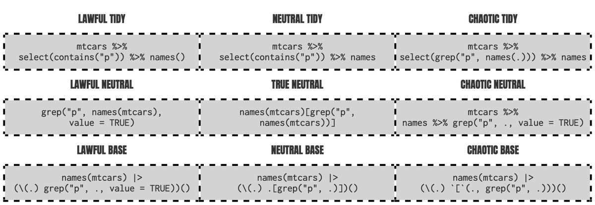
Benefits of base pipe
- Magrittr pipe is bloated with special features which may make it slower than the base pipe
- If not using tidyverse, it’s one less dependency (maybe one day it will be deprecated in tidyverse)
Base pipe with base and anonymous functions
# verbosely
mtcars |> (function(.) plot(.$hp, .$mpg))()
# using the anonymous function shortcut, emulating the dot syntax
mtcars |> (\(.) plot(.$hp, .$mpg))()
# or if you prefer x to .
mtcars |> (\(x) plot(x$hp, x$mpg))()
# or if you prefer to be explicit with argument names
mtcars |> (\(data) plot(data$hp, data$mpg))()
Using “_” placeholder:
mtcars |> lm(mpg ~ disp, data = _)mtcars |> lm(mpg ~ disp, data = _) |> _$coef
Base pipe .[ ] hack
wiki |>
  read_html() |>
  html_nodes("table") |>
  (\(.) .[[2]])() |>
  html_table(fill = TRUE) |>
  clean_names()
# instead of
djia <- wiki %>%
  read_html() %>%
  html_nodes("table") %>%
  .[[2]] %>%
  html_table(fill = TRUE) %>%
  clean_names()
Magrittr, base pipe differences (source)
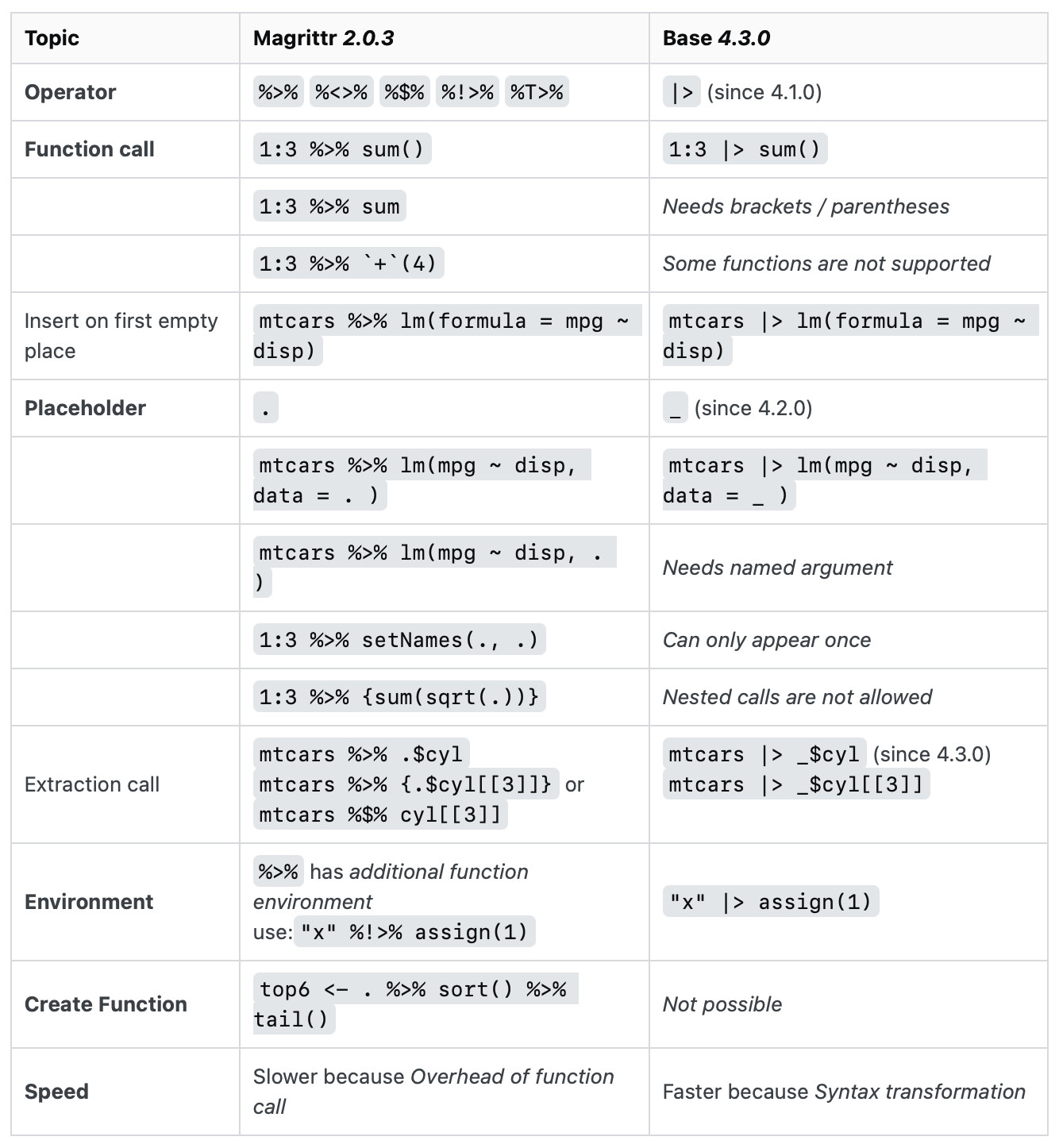
- magrittr:
%>%allows you change the placement with a.placeholder.- base: R 4.2.0 added a
_placeholder to the base pipe, with one additional restriction: the argument has to be named
- base: R 4.2.0 added a
- magrittr: With
%>%you can use.on the left-hand side of operators like$,[[,[and use in multiple arguments (e.g.df %>% {split(.$x, .$y)})- base: can hack this by using anonymous function
- See Base pipe with base and anonymous functions above
- See Base pipe
.[ ]hack above
- base: can hack this by using anonymous function
- magrittr:
%>%allows you to drop the parentheses when calling a function with no other arguments (e.g. dat %>% distinct)- base:
|>always requires the parentheses. (e.g.dat|> distinct()`)
- base:
- magrittr:
%>%allows you to start a pipe with.to create a function rather than immediately executing the pipe
- magrittr:
Purrr with base pipe
data_list |>
  map(\(x) clean_names(x))
# instead of
data_list %>%
  map( ~.x %>% clean_names)
# with split
star |>
  split(~variable) |>
  map_df(\(.) hedg_g(., reading ~ value), .id = "variable")
# instead of
star %>%
  split(.$variable) %>%
  map_df(. %>% hedg_g(., reading ~ value), .id = "variable")
Strings
Resources
- From base R - base R equivalents to {stringr} functions
sprintfx <- 123.456 # Create example data sprintf("%f", x) # sprintf with default specification #> [1] "123.456000" sprintf("%.10f", x) # sprintf with ten decimal places #> [1] "123.4560000000" sprintf("%.2f", x) # sprintf with two rounded decimal places #> [1] "123.46" sprintf("%1.0f", x) # sprintf without decimal places #> [1] "123" sprintf("%10.0f", x) # sprintf with space before number #> [1] " 123" sprintf("%10.1f", x) # Space before number & decimal places #> [1] " 123.5" sprintf("%-15f", x) # Space on right side #> [1] "123.456000 " sprintf("%+f", x) # Print plus sign before number #> [1] "+123.456000" sprintf("%e", x) # Exponential notation #> [1] "1.234560e+02" sprintf("%E", x) # Exponential with upper case E #> [1] "1.234560E+02" sprintf("%g", x) # sprintf without decimal zeros #> [1] "123.456" sprintf("%g", 1e10 * x) # Scientific notation #> [1] "1.23456e+12" sprintf("%.13g", 1e10 * x) # Fixed decimal zeros #> [1] "1234560000000" paste0(sprintf("%f", x), # Print %-sign at the end of number "%") #> [1] "123.456000%" sprintf("Let's create %1.0f more complex example %1.0f you.", 1, 4) #> [1] "Let's create 1 more complex example 4 you."Example: Add leading zeros (source)
numbers <- c(1, 23, 456)
formatted_numbers <- sprintf("%05d", numbers)
print(formatted_numbers)
#> [1] "00001" "00023" "00456"

mixed_input <- c(12, "abc", 345)
formatted_mixed_input <- ifelse(
  is.na(as.numeric(mixed_input)),
  mixed_input,
  sprintf("%05d", as.numeric(mixed_input))
  )
print(formatted_mixed_input)
#> [1] "00012" "abc"   "00345"
str2lang- Allows you to turn plain text into code.growth_rate <- "circumference / age" class(str2lang(growth_rate)) #> [1] "call"Example: Basic
eval(str2lang("2 + 2")) #> [1] 4 eval(str2lang("x <- 3")) x #> [1] 3Example: Run formula against a df
growth_rate <- "circumference / age"
with(Orange, eval(str2lang(growth_rate)))

#>   [1] 0.25423729 0.11983471 0.13102410 0.11454183 0.09748172 0.10349854
#>   [7] 0.09165613 0.27966102 0.14256198 0.16716867 0.15537849 0.13972380
#>  [13] 0.14795918 0.12831858 0.25423729 0.10537190 0.11295181 0.10756972
#>  [19] 0.09341998 0.10131195 0.08849558 0.27118644 0.12809917 0.16867470
#>  [25] 0.16633466 0.14541024 0.15233236 0.13527181 0.25423729 0.10123967
#>  [31] 0.12198795 0.12450199 0.11535337 0.12682216 0.11188369
agrep- Fuzzy Matching (source)Syntax
agrep( pattern, x, max.distance = 0.1, ignore.case = FALSE, value = FALSE, fixed = TRUE )- pattern: The string pattern you want to match
- x: The vector of strings to search within
- max.distance: The maximum allowed distance for a match
- If integer, then the integer is the number of characters that can be wrong
- If decimal, (0,1), then it’s the percentage of characters than can be wrong
- ignore.case: Whether to ignore case when matching
- value: Whether to return the matched values instead of indices
- fixed: Whether to treat the pattern as a fixed string or a regular expression
Examples
- 1
- The first string is missing an “a” and has a “c” where the “k” should be. Therefore, it’s within 2 characters of being correct which equals max.distance, so it gets matched. The output is 1 which indicates the first string.
- 2
- The first string is missing an “a”, has a “c” where the “k” should be, and has a “b” where a “d” should be. Therefore, it’s 3 characters away from being correct which is outside the max.distance. String 2 isn’t close, so nothing gets matched. The output is 0 which indicates the none of the vector indexes has a match.
- 3
- The first string has a “z” where the “s” should be and the second string matches exactly. The max.distance is a quarter of the pattern which is 1 character. Therefore, both strings get matched.
Conditionals
&& and || are intended for use solely with scalars, they return a single logical value.
- Since they always return a scalar logical, you should use && and || in your if/while conditional expressions (when needed). If an & or | is used, you may end up with a non-scalar vector inside if (…) {} and R will throw an error.
& and | work with multivalued vectors, they return a vector whose length matches their input arguments.
Alternative way of negating a condition or set of conditions:
if (!(condition))Makes it less readable IMO, but maybe for a complicated set of conditions if makes more sense in your head to do it this way
Example
if (!(nr == nrow(iris) || (nr == nrow(iris) - 2))) {print("moose")}
Using
else ifif (condition1) { expr1 } else if (condition2) { expr2 } else { expr3 }stopifnotpred_fn <- function(steps_forward, newdata) { stopifnot(steps_forward >= 1) stopifnot(nrow(newdata) == 1) model_f = model_map[[steps_forward]] # apply the model to the last "before the test period" row to get # the k-steps_forward prediction as.numeric(predict(model_f, newdata = newdata)) }%||%Collapse operator which acts like:
`%||%` <- function(x, y) { if (is_null(x)) y else x }- Says if the first (left-hand) input
xisNULL, returny. Ifxis notNULL, return the input
- Says if the first (left-hand) input
Use Cases
Determine whether a function argument is NULL
github_remote <-
  function(repo, username = NULL, ...) {
    meta <- parse_git_repo(repo)
    meta$username <- username %||%
      getOption("github.user") %||%
      stop("Unknown username")
  }
Within the
printargument collapselibrary(rlang) add_commas <- function(x) { if (length(x) <= 1) { collapse_arg <- NULL } else { collapse_arg <- ", " } print(paste0(x, collapse = collapse_arg %||% "")) } add_commas(c("apples")) [1] "apples" add_commas(c("apples", "bananas")) [1] "apples, bananas"
Loops
Misc
next- Proceeds to the next iteration of the loopbreak- Stops the loop
For
If you have to use for-loops, you should pre-allocate memory first to increase performance
# bad result <- c() result <- list() # good result <- numeric(10) # Pre-allocate numeric vector for (i in 1:10) { result[i] <- i^2 } result <- vector("list", n) # Pre-allocate for (i in 1:n) result[[i]] <- i^2Example: List or vector (source)
numbers_list <- list(1, 2, 3, 4, 5) squared_numbers <- vector("list", length(numbers_list)) for (i in seq_along(numbers_list)) { squared_numbers[[i]] <- numbers_list[[i]]^2 } print(squared_numbers)Example: Number Range and Nested
# 2x3
x <- matrix(1:6, 2, 3)

for (i in seq_len(nrow(x))) {
  for(j in seq_len(ncol(x))) {
    print(x[i, j])
  }
}
While
Example (source)
numbers_list <- list(2, 4, 6, 8, 10, 12, 14)
index <- 1

while (numbers_list[[index]] <= 10) {
  index <- index + 1
}

print(paste("The first number greater than 10 is:", numbers_list[[index]]))
tapplytapply(mtcars$mpg, mtcars$cyl, FUN = mean) #> 4 6 8 #> 26.66364 19.74286 15.10000
Columns
Change the names of all columns
colnames(df) <- c("good", "better")Change the name of 1 column
colnames(df)[1] <- "NOX_ID"- Changes 1st column’s name to NOX_ID
Sorting/Ordering
Ascending:
df[with(df, order(col2)), ] # or df[order(df$col2), ] # or sort_by(df, df$col2)- col2 is the column used to sort the df by
Descending:
df[with(df, order(-col2)), ]By Multiple Columns
- Sequentially:
sort_by(df, df$col1, df$col2, df$col3)- Says sort by col1 then col2 then col3
- Descending then Ascending:
df[with(df, order(-col2, id)), ]
- Sequentially:
Move the 3rd column of a matrix/df to the 1st column
mat_new <- mat[, c(3, setdiff(seq_len(ncol(mat)), 3))]
Change position of columns
# Reorder column by index manually
df2 <- df[, c(5, 1, 4, 2, 3)]
df3 <- df[, c(1, 5, 2:4)]
# Reorder column by name manually
new_order = c("emp_id","name","superior_emp_id","dept_id","dept_branch_id")
df2 <- df[, new_order]
Set Operations
Unique values in A that are not in B
a <- c("thing", "object") b <- c("thing", "gift") unique(a[!(a %in% b)]) #> [1] "object" setdiff(a, b)setdiffis slower
Unique values of the two vectors combined
unique(c(a, b)) #> [1] "thing" "object" "gift" union(a, b)unionis just a wrapper forunique
Subsetting
Lists and Vectors
Removing Rows
# Remove specific value from vector
x[!x == 'A']

# Remove multiple values by list
x[!x %in% c('A', 'D', 'E')]

# Using setdiff
setdiff(x, c('A','D','E'))

# Remove elements by index
x[-c(1,2,5)]

# Using which
x[-which(x %in% c('D','E') )]

# Remove elements by name
x <- c(C1='A',C2='B',C3='C',C4='E',C5='G')
x[!names(x) %in% c('C1','C2')]
Dataframes
Remove specific Rows
df <- df[-c(25, 3, 62), ]Remove column by name
df <- df[, which(names(df) == "col_name")]
df <- subset(df, select = -c(col_name))
df <- df[, !names(df) %in% c("col1", "col2"), drop = FALSE]
Filter and Select
df <-
  subset(df,
         subset = col1 > 56,
         select = c(col2, col3))
Value Replacement
Replace NAs in one df with values from another df
tib1$latitude[tib1$name == "Bob"] <- tib2[tib2$name == "Bob", "lat"] tib1$longitude[tib1$name == "Bob"] <- tib2[tib2$name == "Bob", "long"]- Also see R, Tidyverse >> dplyr >>
rows_update - tib1 has NAs for Bob’s latitude and longitude
- tib2 has values in lat and long for Bob’s latitude and longitude
- Also see R, Tidyverse >> dplyr >>
Transformation
Example:
transformandsubset(source)mtcars |> transform(avg = mpg / wt) |> subset(avg > 5) |> subset(, c(wt, mpg, avg))transformcannot refer to variables previously created in the same transformation. You’d be required to use an additional transform in order to use that variable.See Functions >>
withinfor an alternate method
Joins
- Inner join:
inner <- merge(flights, weather, by = mergeCols) - Left (outer) join:
left <- merge(flights, weather, by = mergeCols, all.x = TRUE) - Right (outer) join:
right <- merge(flights, weather, by = mergeCols, all.y = TRUE) - Full (outer) join:
full <- merge(flights, weather, by = mergeCols, all = TRUE) - Cross Join (Cartesian product):
cross <- merge(flights, weather, by = NULL) - Natural join:
natural <- merge(flights, weather)
Error Handling
stopExample:
switch(parallel, windows = "snow" -> para_proc, other = "multicore" -> para_proc, no = "no" -> para_proc, stop(sprintf("%s is not one of the 3 possible parallel argument values. See documentation.", parallel)))- parallel is the function argument. If it doesn’t match one of the 3 values, then an error is thrown.
tryIf something errors, then do something else
Example
current <- try(remDr$findElement(using = "xpath", '//*[contains(concat( " ", @class, " " ), concat( " ", "product-price-value", " " ))]'), silent = T) #If error : current price is NA if(class(current) =='try-error'){ currentp[i] <- NA } else { # do stuff }Example: Geospatial, Spatio-Temporal >> EDA >> Spatial Dependence >> Example 1
vario_mod <- try(
  fit.variogram(
    vario_exp,
    vgm(psill = 100,
        "Exp",
        range = 200)),
  silent = TRUE
)

if (inherits(vario_mod, "try-error"))
  return(c(NA, NA))
tryCatchRun the main code, but if it “catches” an error, then the secondary code (the workaround) will run.
Example 1: Basic
tryCatch(
  # try to evaluate the expression
  {
    log("a")
  },

  # what happens if there's a warning?
  warning = function(w) {
    print("There was a warning. Here's the message:")
    print(w)
  },

  # what happens if there's an error?
  error = function(e) {
    print("There was an error. Returning `NA`.")
    return(NA)
  }
)
Example 2: Logging 1
err_pkgs <- list() for (i in seq_along(moose)) { print(moose[i]) tryCatch( expr = pak::pkg_install(moose[i], ask = FALSE), error = function(e) { err_pkgs[[i]] <<- moose[i] } ) }- Stores the names of packages that don’t get installed into err_pkgs
- Note the super-assignment used so that the error function can find err_pkgs
- Needed since err_pkgs is being modified and not just called
Example 3: Logging 2 (source)
OUTPUT_DIR <- "reports"

# Create output directory
if (!dir.exists(OUTPUT_DIR)) {
  dir.create(OUTPUT_DIR, recursive = TRUE)
  cat(sprintf("Created output directory: %s\n", OUTPUT_DIR))
}

# Initialize logging
log_file <- file.path(
  OUTPUT_DIR,
  sprintf("burst-report-log_%s.txt", format(Sys.time(), "%Y%m%d_%H%M%S"))
)
log_conn <- file(log_file, open = "wt")

log_msg <- function(msg, level = "INFO") {
  timestamp <- format(Sys.time(), "%Y-%m-%d %H:%M:%S")
  log_line <- sprintf("[%s] %s: %s", timestamp, level, msg)
  cat(log_line, "\n", file = log_conn)
  cat(log_line, "\n")
}

tryCatch(
  {
    # some code
  },
  error = function(e) {
    # Clean up temp directory on error
    if (dir.exists(temp_dir)) {
      unlink(temp_dir, recursive = TRUE)
    }

    error_msg <- sprintf(
      "Failed for store %d (%d-%02d): %s",
      store_key,
      year,
      month,
      e$message
    )
    log_msg(error_msg, "ERROR")
  }
)
Example 4: Basic in a for-loop
for (r in 1:nrow(res)) { cat(r, "\n") tmp_wikitext <- get_wikitext(res$film[r], res$year[r]) # skip if get_wikitext fails if (is.na(tmp_wikitext)) next if (length(tmp_wikitext) == 0) next # give the text to openai tmp_chat <- tryCatch( get_results(client, tmp_wikitext), error = \(x) NA ) # if openai returned a dict of 2 if (length(tmp_chat) == 2) { res$writer[r] <- tmp_chat$writer res$producer[r] <- tmp_chat$producer } }get_resultsis called during each iteration, and if there’s an error a NA is returned.
Example 5:
pct_difference_error_handling <- function(n1, n2) { # Try the main code tryCatch(pct_diff <- (n1-n2)/n1, # If you find an error, use this code instead error = return( cat( 'The difference between', as.integer(n1), 'and', as.integer(n2), 'is', (as.integer(n1)-as.integer(n2)), 'which is', 100*(as.integer(n1)-as.integer(n2))/as.integer(n1), '% of', n1 )#cat ), # finally = print('Code ended') # optional )#trycatch # If no error happens, return this statement return ( cat('The difference between', n1, 'and', n2, 'is', n1-n2, ', which is', pct_diff*100, '% of', n1) ) }- Assumes the error will be the user enters a string instead of a numeric. If errors, converts string to numeric and calcs.
- “finally” - This argument will always run, regardless if the try block raises an error or not. So it could be a completion message or a summary, for example.
Example 6: Save output; Model fitting (source >> Starting Values >> Example 1)
fit_ssm <- tryCatch({ fit.StVariogram( vario_emp, mod, fit.method = wgt, stAni = num_stani_mat, # get rid of "range should be positive" error lower = c( sill.s = 0, range.s = 1, # km sill.t = 0, range.t = 0.1, # days sill.st = 0, range.st = 1, nugget = 0, anis = 1 ), control = list(maxit=10000) ) }, error = \(e) { message( "kappa = ", k, " and weight method = ", wgt, " failed: ", e$message ) return(NULL) }) if (is.null(fit_ssm)) return(NULL) attr_opt <- attributes(fit_ssm)$optim.output tib_res <- tibble( kappa = k, weight_method = wgt, fit_ssm = list(fit_ssm), converge = attr_opt$convergence, message = attr_opt$message, sse = attr_opt$value ) return(tib_res)- This chunk of code is from inside a function — hence the
returnfunctions - By saving the output of the
tryCatch, I can return a NULL. Therefore, in the final resultant tibble, there won’t be any evidence of this fitted object or its error. - There will be a message in console about the parameter settings that lead to the error and the error message itself.
- This chunk of code is from inside a function — hence the
Models
formulaandupdateform <- formula(log(median) ~ CRIM + ZN + INDUS + CHAS + I((NOX*10)^2) + I(RM^2) + AGE + log(DIS) + log(RAD) + TAX + PTRATIO + I(BB/100) + log(I(LSTAT/100))) MLM <- lmer(update(form, . ~ . + (1 | NOX_ID)), data = boston_487, REML = FALSE)reformulate- Create formula sytax programmatically# Creating a formula using reformulate() formula <- reformulate(c("hp", "cyl"), response = "mpg") # Fitting a linear regression model model <- lm(formula, data = mtcars) formula ##> mpg ~ hp + cyl- Can also use
as.formula
- Can also use
DF2formula- Turns the column names from a data frame into a formula. The first column will become the outcome variable, and the rest will be used as predictorsDF2formula(Orange) #> Tree ~ age + circumferenceformula- Provides a way of extracting formulae which have been included in other objectsrec_obj |> prep() |> formula()- Where “rec_obj” is a tidymodels recipe object
Data from Model Object
model$modelreturn the data dataframedeparse(model$call$data)gives you that name of your data object as a string.model$call$datagives you the data as an unevaluated symbol;
eval(model$call$data)gives you back the original data object, if it is available in the current environment.