Linear
Misc
Guide for suitable baseline models: link
“For estimation of causal effects, it does typically not suffice to well control for confounders, we also need a sufficiently strong source of exogenous variation for our explanatory variable of interest.”
- From Empirical Economics with R: Confounders, Proxies, and Sources of Exogenuous Variations
- Even if you have good proxy variables for the true confounder(s) and use them as controls, estimated effects of explanatory variables with low s.d. (with mean = 0, e.g. low 0.02, high 1) will still be inflated If the regression conditions aren’t met - for instance, if heteroskedasticity is present - then the OLS estimator is still unbiased but it is no longer best. Instead, a variation called generalized least squares (GLS) will be Best Linear Unbiased Estimator (BLUE)
A model is said to be hierarchical if it contains all the lesser degree terms in the hierarchy
- Example
- hierarchical: y = x + x2 + x3 + x4
- not hierarchical: y = x + x4
- hierarchical: y = x1 + x2 + x1x2
- not hierarchical: y = x1 + x1x2
- It is expected that all polynomial models should have this property because only hierarchical models are invariant under linear transformation.
- Example
Specifying Nonlinear terms
Use
poly(x, 2)if:- You want orthogonal contrasts (e.g., for ANOVA-style inference).
- Your predictor is an ordered factor (e.g., “Low”, “Medium”, “High”).
- You care about hypothesis testing (e.g., “Is there a significant quadratic trend?”).
Use
x + I(x^2)if:- Your predictor is numeric and you want a traditional polynomial regression.
- You don’t care about orthogonality.
- You can use this method and avoid collinearity by centering your variable first (source)
- Interpretation of raw coefficients is needed.
RcppArmadillo::fastLmPureNot sure what this does but it’s rcpp so maybe faster than lm for big data..lm.fitis a base R lm function that is 30%-40% faster than lm.Various Specifications
# 1 interaction
lm(Y ~ D*X1, data = dat)
# or
lm(Y ~ D + X1 + D*X1, data = dat)

# 2 interactions
lm(Y ~ D * (X1 + X2), data = dat)
# or
lm(Y ~ D + X1 + X2 + D*X1 + D*X2, data = dat)
Assumptions
- Assumptions
- The true relationship is linear
- i.e. a linear relationship between the independent variable, x, and the dependent variable, y.
- Errors are normally distributed
- i.e. random fluctuations around the true line
- Homoscedasticity of errors (or, equal variance around the line)
- i.e. variability in the response doesn’t increase as the value of the predictor increases
- Independence of the observations
- i.e. no autocorrelation
- The true relationship is linear
- Check residuals
- have a constant variance (Homoscedasticity of errors)
- be approximately normally distributed (with a mean of zero) (Errors are normally distributed)
- be independent of one another (independence, no autocorrelation)
- Gelman’s order of importance (post)
- Validity. Most importantly, the data you are analyzing should map to the research question you are trying to answer. This sounds obvious but is often overlooked or ignored because it can be inconvenient
- Additivity and linearity. The most important mathematical assumption of the regression model is that its deterministic component is a linear function of the separate predictors
- Independence of errors
- Equal variance of errors
- Normality of errors - “Normality and equal variance are typically minor concerns, unless you’re using the model to make predictions for individual data points.”
EDA
- Preliminary
- Set seed
- Check for missing values
- See how many predictors you’re allowed to use given the sample size. Check bkmk: statistics –> sample size folder for Harrell articles
- remove predictors with zero variance recipes::step_zv(all_predictors()).
- Check correlation matrix. greybox::assoc()
- Check s.d. in predictors
- without enough variation in predictors (with mean = 0, e.g. low sd = 0.02, high = 1), effects will be inflated even after controlling for potential confounders
- Look at series of pairwise plots: see which independent variables are linearly related to your dependent variable as they would be good predictors. Also look for non-linearity relations. See which of your independent variables are linearly related to each other as this indicates collinearity. Use greybox::spread w/log = false for linear relationships and log = true for nonlinear
- Collinearity can cause sign flips of coefficients as variables are added or taken away when we create our model. Use vif() and greybox::determ pg 121
- In pairwise for prospective predictors, look for and make note of potential outlier points.
- Look at histograms of variables to check for skewness. We want normal distributions but distributions that are all similarly skewed isn’t too bad either.
- Look at summary statistics and examine the difference between the median and the mean as this indicates skewness.
- Skewness metric?
- Look at box plots to check for skewness and outliers. Investigate at outliers to see if they can be removed as they can have an outsized effect that causes inaccuracy in your model.
- Is the outcome variable is multi-modal?
- Regression, Other
- Solutions:
- Quantile Regression (See Regression, Quantile)
- Mixture models
Transformations
- Misc
- Standardization
- Methods
- {effectsize}
- Can also be used to standardize coefficients after the model has been fit
- Can also be done by multiplying the coefficient by the sd of the variable
- Good docs - applications, reliability, etc. of the many methods for mixed models, interaction terms are explained.
- Can also be used to standardize coefficients after the model has been fit
- Centering and Scaling
- median and MAD
- robust
- Mean and (2 ⨯ std dev)
- Gelman (2008)
- Allows for factor variables to also be compared to numeric variables in terms of importance
- Median and IQR
- Mean and Gini Mean Difference
- {effectsize}
- Methods
- Scaling
- var/max(var)
- Making the largest value = 1 and the theoretical minimum = 0
- var/max(var)
- Squaring (quadratic)
- Predictors should be standardized.
- Squaring variables can produce some very large numbers and the numerical estimations of the effects can be get screwed up.
- Centering fixes collinearity issues when creating powers and interaction terms (CV post)
- Collinearity between the created terms and the main effects
- Predictors should be standardized.
- Log
- Taking the log of a measure translates the measure into magnitudes. So by using the logarithm of a predictor, we’re saying that we suspect that the magnitude of the predictor is related to outcome, in a linear fashion.
- Logging the response should only be used if you’re trying fix heteroskedacity in the residuals. Otherwise, a gaussian glm with log link should be used. (StackExchange, Paper)
Contrasts
Misc
- In statistical modeling (like ANOVA or linear regression), categorical variables (factors) need to be “coded” numerically so that they can be included in the model. This coding is done via contrast matrices. Different contrast schemes allow you to test different types of hypotheses about the differences between factor levels.
- Notes from Centering in Moderation Analysis: A Guide
- Resource
- Not Another Post Hoc Paper: A New Look at Contrast Analysis and Planned Comparisons
- A tutorial on:
- How planned contrasts work
- Which kinds of contrasts can be used
- How to set customized contrasts
- How to obtain the R code for such contrasts for both simple and interaction effects.
- Includes a Shiny App called “appRiori” to make each step understandable and reproducible.
- A tutorial on:
- Not Another Post Hoc Paper: A New Look at Contrast Analysis and Planned Comparisons
Three Ways to Change Contrasts
# 1. assign to the contrasts() function
contrasts(data$G) <- contr.sum

# 2. The C() function (BIG C!)
data$G <- C(data$G, contr = contr.sum)

# 3. In the model
lm(Y ~ G,
   data = data,
   contrasts = list(G = contr.sum))
Treatment Contrasts
Default contrasts used by R,
stats::contr.treatment()For a factor variable, it constructs each dummy variable to be 0 for all but the first level of the factor, with the 1st level being left out.
Example: Dummy variables for a factor variable with 3 levels
contr.treatment(levels(data$G)) #> g2 g3 #> g1 0 0 #> g2 1 0 #> g3 0 1- Where g1 is the reference level.
Example: Interpretation for a factor variable with 3 levels
parameters::model_parameters(model) #> Parameter | Coefficient | SE | 95% CI | t(7) | p #> ------------------------------------------------------------------- #> (Intercept) | 23.33 | 0.96 | [ 21.05, 25.61] | 24.21 | < .001 #> G [g2] | -3.19 | 1.22 | [ -6.08, -0.31] | -2.62 | 0.034 #> G [g3] | -6.83 | 1.52 | [-10.44, -3.23] | -4.49 | 0.003 (predicted_means <- predict(model, newdata = data.frame(G = c("g1", "g2", "g3")))) #> 1 2 3 #> 23.33333 20.14000 16.50000 predicted_means[2] - predicted_means[1] #> 2 #> -3.193333 predicted_means[3] - predicted_means[1] #> 3 #> -6.833333- Shows how the dummy variable coefficients are the difference in predicted means between a given factor level and the reference level.
Sum-to-Zero Contrasts
The intercept represents the grand mean which is the average of all group means of the factor variable.
Example: Factor variable with 3 levels
contr.sum(levels(data$G)) #> [,1] [,2] #> g1 1 0 #> g2 0 1 #> g3 -1 -1Example: Interpretation for a factor variable with 3 levels
model_parameters(model7) #> Parameter | Coefficient | SE | 95% CI | t(7) | p #> ------------------------------------------------------------------ #> (Intercept) | 19.99 | 0.57 | [18.65, 21.33] | 35.35 | < .001 #> G [1] | 3.34 | 0.79 | [ 1.47, 5.22] | 4.21 | 0.004 #> G [2] | 0.15 | 0.71 | [-1.53, 1.83] | 0.21 | 0.840 (predicted_means <- predict(model6, newdata = data.frame(G = c("g1", "g2", "g3")))) #> 1 2 3 #> 23.33333 20.14000 16.50000 predicted_means[1] - mean(predicted_means) #> 1 #> 3.342222 predicted_means[2] - mean(predicted_means) #> 2 #> 0.1488889- Each factor level coefficient is the difference between that level’s group mean and the grand mean.
Example: Continuous and Categorical Predictors With Interaction
model12 <- lm(Y ~ Q * A, data = data, contrasts = list(A = contr.sum)) model_parameters(model12) #> Parameter | Coefficient | SE | 95% CI | t(6) | p #> ------------------------------------------------------------------ #> (Intercept) | 4.98 | 6.79 | [-11.63, 21.59] | 0.73 | 0.491 #> Q | 4.27 | 1.91 | [ -0.39, 8.94] | 2.24 | 0.066 #> A [1] | -7.38 | 6.79 | [-23.99, 9.23] | -1.09 | 0.319 #> Q × A [1] | 1.70 | 1.91 | [ -2.96, 6.37] | 0.89 | 0.406 # Predict for all combinations of Q = [0, 1] and A = [a1, a2] pred_grid <- expand.grid(Q = c(0, 1), A = c("a1", "a2")) (predicted_means <- predict(model11, newdata = pred_grid)) #> 1 2 3 4 #> -2.400173 3.574452 12.358596 14.929210 # Average slope of X mean(c(predicted_means[2] - predicted_means[1], predicted_means[4] - predicted_means[3])) #> [1] 4.272619- \(Q\) is continuous while \(A\) is a two-level factor variable.
- The main effect for \(Q\) is called the Grand Average Slope.
Deviation Contrasts
Combination of Treatment Contrasts and Sum-to-Zero Contrasts
- Coefficients are the same as in Treatment Contrasts
- Intercept is the grand mean as in Sum-to-Zero Contrasts
Available via {datawizard::contr.deviation}
Example:
model8 <- lm(Y ~ G,
             data = data,
             contrasts = list(G = contr.deviation))

model_parameters(model8)
#> Parameter   | Coefficient |   SE |          95% CI |  t(7) |      p
#> -------------------------------------------------------------------
#> (Intercept) |       19.99 | 0.57 | [ 18.65, 21.33] | 35.35 | < .001
#> G [g2]      |       -3.19 | 1.22 | [ -6.08, -0.31] | -2.62 | 0.034
#> G [g3]      |       -6.83 | 1.52 | [-10.44, -3.23] | -4.49 | 0.003

(predicted_means <- predict(model6,
                            newdata = data.frame(G = c("g1", "g2", "g3"))))
#>        1        2        3
#> 23.33333 20.14000 16.50000
mean(predicted_means)
#> [1] 19.99111
predicted_means[2] - predicted_means[1]
#>         2
#> -3.193333
predicted_means[3] - predicted_means[1]
#>         3
#> -6.833333
Polynomial Contrasts
Contructed to look for specific patterns in the means of the groups that correspond to polynomial functions.
Useful when you suspect a non-linear (polynomial) relationship between an ordinal factor (e.g., ordered levels like “Low,” “Medium,” “High”) and the response variable in linear model
- Assumes the levels of the ordered factor as corresponding to equally spaced values of an underlying continuous covariate.
- I think if the number of observations for each level is not balanced, then it indicates that the levels aren’t equally spaced. (See example)
- If this assumption is not met, it’s recommended to use {codingMatrices::contr.diff} which operates like
contr.treatment; the contrasts are then contrasts of the succeeding category mean with the mean of the preceding category. (See example)
- Assumes the levels of the ordered factor as corresponding to equally spaced values of an underlying continuous covariate.
The contrasts are constructed such that they are orthogonal (uncorrelated), meaning each polynomial term (linear, quadratic, cubic, etc.) provides independent information.
For a factor with k levels,
contr.poly(k)generates (k-1) orthogonal polynomial contrasts (linear, quadratic, cubic, etc.).stats::contr.poly(n, scores = NULL, contrasts = TRUE)n: The number of levels in your factor.scores: (Optional) A numeric vector of scores associated with each level. IfNULL(the default),contr.polyassumes equally spaced levels (1, 2, …, n). If your levels are not equally spaced (e.g., 10mg, 20mg, 50mg), you should provide the actual scores.contrasts: A logical value indicating whether contrasts should be computed (default isTRUE). IfFALSE, a square matrix is returned.
Example: View contrasts
ordered_factor <- ordered(c("Low", "Medium", "High")) contrasts(ordered_factor) <- contr.poly(3) ordered_factor #> .L .Q #> Low -7.071068e-01 0.4082483 #> Medium -7.850462e-17 -0.8164966 #> High 7.071068e-01 0.4082483 #> Levels: High < Low < Medium- .L = Linear contrast
- .Q = Quadratic contrast
Example: Test for nonlinear relationship
Data and Model
set.seed(123) # For reproducibility # Simulate data with a quadratic trend n <- 30 dosage <- ordered(rep(c("Low", "Medium", "High"), each = n/3), levels = c("Low", "Medium", "High")) response_ms <- c( rnorm(n/3, mean = 200, sd = 20), # Low dose rnorm(n/3, mean = 180, sd = 15), # Medium dose rnorm(n/3, mean = 210, sd = 25) # High dose (U-shaped trend) ) dat <- data.frame(dosage, response_ms) dat <- data.frame(dosage, response_ms) contrasts(dat$dosage) <- contr.poly(nlevels(dat$dosage)) # 3 levels → Linear (.L) & Quadratic (.Q) mod <- lm(response_ms ~ dosage, data = dat) summary(mod) #> Estimate Std. Error t value Pr(>|t|) #> (Intercept) 200.617 3.043 65.930 < 2e-16 *** #> dosage.L 6.436 5.270 1.221 0.233 #> dosage.Q 25.411 5.270 4.821 4.92e-05 ***- dosage.Q (Quadratic, p = 1.19e-05): Strong quadratic trend
- So you probably want include
poly(dosage, 2)in your model
Show Trend
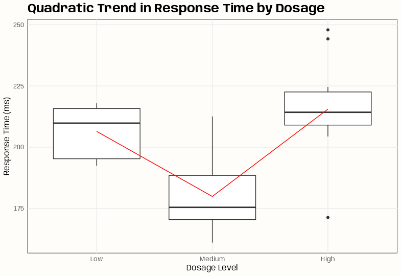
ggplot(dat, aes(x = dosage, y = response_ms)) + geom_boxplot() + stat_summary(fun = mean, geom = "line", aes(group = 1), color = "red") + labs(title = "Quadratic Trend in Response Time by Dosage", x = "Dosage Level", y = "Response Time (ms)") + theme_notebook()- U-shaped effect: Medium dose has the lowest response time.
Example:
contr.diff(source)library(codingMatrices) fhouse <- cut(eng324$house, c(0.0, 0.25, 0.90, 1)) table(fhouse) ## fhouse ## (0,0.25] (0.25,0.9] (0.9,1] ## 1 23 300 fhouse <- as.ordered(fhouse) attr(C(fhouse), "contrasts") ## ordered ## "contr.poly" contrasts(fhouse) <- "contr.diff" attr(fhouse, "contrasts") ## [1] "contr.diff" contrasts(fhouse) ## m2-m1 m3-m2 ## 1 0 0 ## 2 1 0 ## 3 1 1 eng324$fhouse <- fhouse- fhouse is a binned version of the house variable, which is the proportion of garbage pick-up points that are residential, rather than business
- When used in a linear regression, you get coefficients for the m2 - m1 and m3 - m2. So the coefficients are a comparison between the means of level 2 and level 1 and a comparison between the means of level 3 and level 2.
Model Selection
- Harrell says use all variables unless number of variables , p > (nrow(df) / 15), then use Regularized Regression
- See Harrell sample size biostat paper (above). Has overview of approaches (I think).
- Use best subsets with Mallow’s CP, AIC, and BIC as metrics for choosing best model. See R notebook, pg 121 and bkmk regression \(\rightarrow\) multivariable folder for PSU stat 501
- Check for partial correlations between predictor variables and outcome variable (see notebook and bookmarks) as a possible avenue of feature reduction and as a way of gauging true strength of the relationship between the predictor variables and outcome variable
Interpretation
- Marginal Effect - The effect of the predictor after taking into account the effects of all the other predictors in the model
summaryStandard Errors: An estimate of how much estimates would ‘bounce around’ from sample to sample, if we were to repeat this process over and over and over again.
- More specifically, it is an estimate of the standard deviation of the sampling distribution of the estimate.
t-stat: Ratio of parameter estimate and its SE
- used for hypothesis testing, specifically to test whether the parameter estimate is ‘significantly’ different from 0.
p-value: The probability of finding an estimated value that is as far or further from 0, if the null hypothesis were true.
Note that if the null hypothesis is not true, it is not clear that this value is telling us anything meaningful at all.
Example: Manual Calculation
# predictor
predictor <- "d"

# number of cases
n <- nrow(dat)

#number of model terms
p <- nrow(model$coefficients)

# one-tailed p-value
# q = absolute t-value
# df = degrees of freedom
p_value_one_tailed <- stats::pt(
  q = abs(model$coefficients[predictor, "t value"]),
  df = n - p #degrees of freedom
  )

#two-tailed p-value
2 * (1 - p_value_one_tailed)
F-statistic: This “simultaneous” test checks to see if the model as a whole predicts the response variable better than chance alone.
- i.e. whether or not all the estimates should be considered unable to be differentiated from 0
- If this statistic’s p-value < 0.05, then this suggests that at least some of the parameter estimates are not equal to 0
- Unless you only have an intercept model, you have multiple tests (e.g. variables + intercept p-values). There is no protection from the problem of multiple comparisons without this.
- Bear in mind that because p-values are random variables–whether something is significant would vary from experiment to experiment, if the experiment were re-run–it is possible for these to be inconsistent with each other.
Residual Standard Error
\[ \hat \sigma = \frac{\sum (e^2)}{\mbox{dof}} \]
- \(\sum (e^2)\) is the Residual Sum of Squares (RSS)
- \(\mbox{dof}\) are the residual degrees of freedom which is number of rows of the dataset - number of parameters estimated. e.g. \(\hat Y_i = \beta_0 + \beta_1X_i + e_i\) would have two parameters to estimate (\(\beta_0\), \(\beta_1\)).
- The rule of thumb is 20 dof to have a reasonably small residual standard error (10 dof at least).
- Mixed Effects models typically have lower dof due to their complexity but it’s acceptable given that they’re able to better account for the dependence structure.
- Intercept
- If variables are centered so that the predictors have mean 0, this is the expected value of Yi when the predictor values are set to their means.
- If variables are not centered so that the predictors have mean 0, this is the expected value of Yi when the predictors are set to 0.
- may not be a realistic or interpretable situation (e.g. what if the predictors were height and weight?)
- Standardized Predictors
- Dimensions are in common units (standard deviations), and the
- Coefficients
- Similar to Pearson Correlation Coefficients (r-scores)
- Can’t be compared to other standardized coefficients to determine importance
- Unless the “true” r-score value is zero, the estimate is driven in large part by the range of values of the predictor in the sample
- The best that can ever be said is that variability in one explanatory variable within a specified range is more important to determining the level of the response than variability in another explanatory variable within another specified range
- “variability” makes sense since the units are standard deviations
- Trying to interpret these coefficients in terms of “importance” is probably not practically useful then.
- Unless the data is large and/or the range of the predictors is representative of the population
- Does one coefficient have a larger effect than the other?
Example: does extra hours work have a statistically larger effect on salary than does number_compliments_to_the_boss
library(parameters)
library(effectsize)
data("hardlyworking", package = "effectsize")
hardlyworkingZ <- standardize(hardlyworking)
m <- lm(salary ~ xtra_hours + n_comps, data = hardlyworkingZ)
model_parameters(m)
#> Parameter  | Coefficient |  SE |        95% CI |    t(497) |      p
#> ---------------------------------------------------------------------
#> (Intercept) |  -7.19e-17 | 0.02 | [-0.03, 0.03] | -4.14e-15 | > .999
#> xtra_hours  |        0.81 | 0.02 | [ 0.78, 0.84] |    46.60 | < .001
#> n_comps    |        0.41 | 0.02 | [ 0.37, 0.44] |    23.51 | < .001

# method 1
# assume both variables have same coeff and test if the models are different
m0 <- lm(salary ~ I(xtra_hours + n_comps), data = hardlyworkingZ)
model_parameters(m0)
anova(m0, m) # Yes they are different and therefore xtra_hours does have a stronger effect
#> Analysis of Variance Table
#>
#> Model 1: salary ~ I(xtra_hours + n_comps)
#> Model 2: salary ~ xtra_hours + n_comps
#>  Res.Df    RSS Df Sum of Sq      F    Pr(>F)
#> 1    498 113.67
#> 2    497  74.95  1    38.716 256.73 < 2.2e-16 ***

# method 2
library(car)
linearHypothesis(m, c("xtra_hours - n_comps"))
#> Linear hypothesis test
#>
#> Hypothesis:
#> xtra_hours - n_comps = 0
#>
#> Model 1: restricted model
#> Model 2: salary ~ xtra_hours + n_comps
#>
#>  Res.Df    RSS Df Sum of Sq      F    Pr(>F)
#> 1    498 113.67
#> 2    497  74.95  1    38.716 256.73 < 2.2e-16 ***

# method 3
library(emmeans)
trends <- rbind(
  emtrends(m, ~1, "xtra_hours"),
  emtrends(m, ~1, "n_comps")
)
# clean up so it does not error later
trends@grid# Regression, Gaussian

1` <- c("xtra_hours", "n_comps")
trends@misc$estName <- "trend"

trends
#>  1          trend    SE  df lower.CL upper.CL
#>  xtra_hours 0.811 0.0174 497    0.772    0.850
#>  n_comps    0.409 0.0174 497    0.370    0.448
#>
#> Confidence level used: 0.95
#> Conf-level adjustment: bonferroni method for 2 estimates

pairs(trends)
#>  contrast            estimate    SE  df t.ratio p.value
#>  xtra_hours - n_comps    0.402 0.0251 497 16.023  <.0001
- Quadratic
- µi = α + β1xi + β2xi2
- α is the intercept. Tells us the expected value of µ when x is 0
- β1 and β2 are linear and square components of the regression curve, respectively
- µi = α + β1xi + β2xi2
Report
- Outliers
- List any outliers that were removed and reasons why.
- Report results with and without outliers
- Coefficients with uncertainty
Example: Basic (source)
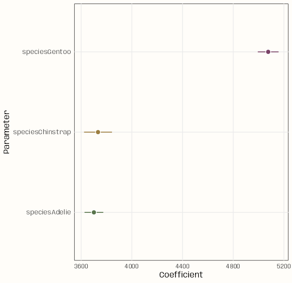
library(ggplot2) library(parameters) notebook_colors <- unname(swatches::read_ase( here::here("palettes/Forest Floor.ase") )) lm(body_mass ~ 0 + species, data = penguins) |> model_parameters() |> ggplot(aes( x = Coefficient, y = Parameter)) + geom_linerange(aes( xmin = CI_low, xmax = CI_high, color = Parameter)) + geom_point( aes(fill = Parameter), size = 3, shape = 21, color = "white") + scale_color_manual(values = notebook_colors[c(4,7,9)]) + scale_fill_manual(values = notebook_colors[c(4,7,9)]) + guides(color = "none", fill = "none") + theme_notebook()library(ggplot2) library(parameters) library(ggdist) notebook_colors <- unname(swatches::read_ase( here::here("palettes/Forest Floor.ase") )) lm(body_mass ~ 0 + species, data = penguins) |> model_parameters() |> ggplot(aes(x = Coefficient, y = Parameter)) + geom_pointinterval( aes( xmin = CI_low, xmax = CI_high, interval_color = Parameter, point_fill = Parameter ), shape = 21, point_color = "white", point_size = 3 ) + scale_color_manual( aesthetics = "interval_color", values = notebook_colors[c(4,7,9)]) + scale_fill_manual( aesthetics = "point_fill", values = notebook_colors[c(4,7,9)]) + guides(interval_color = "none", point_fill = "none") + theme_notebook()
Linear Algebra
Notes from Matrix Algebra for Educational Scientists, Chapters 27, 29
- Also has R code for calculations and extracting values from models
Model Formula
\[ \begin{align} \boldsymbol{y} &= \boldsymbol{X}\beta+ \boldsymbol{\epsilon} \\ \beta &= (\boldsymbol{X}^T \boldsymbol{X})^{-1} \boldsymbol{X}^T \boldsymbol{y} \\ \end{align} \]
Fitted Values and Hat Matrix
\[ \begin{align} \boldsymbol{\hat{y}} &= \boldsymbol{X}\beta \\ &= \boldsymbol{X}(\boldsymbol{X}^T\boldsymbol{X})^{-1} \boldsymbol{X}^T \boldsymbol{y} \\ &= \boldsymbol{H} \boldsymbol{y} \end{align} \]
- The number of parameters being estimated by the model is the trace of the hat matrix, \(\text{tr}(H)\)
Residuals
\[ \begin{align} \boldsymbol{\epsilon} &= \boldsymbol{y} - \boldsymbol{\hat{y}} \\ &= \boldsymbol{y} - \boldsymbol{H}\boldsymbol{y} \\ &= (\boldsymbol{I}-\boldsymbol{H})\boldsymbol{y} \end{align} \]
Residual Variance
\[ \hat{\sigma}^2_\epsilon = \frac{\boldsymbol{\epsilon}^T\boldsymbol{\epsilon}}{n - \mbox{tr}(\boldsymbol{H})} \]
Coefficient Covariance Matrix
\[ \begin{align} \boldsymbol{\sigma}_\beta^2 &= \sigma_\epsilon^2 (\boldsymbol{X}^T \boldsymbol{X})^{-1} \\ &= \begin{bmatrix} \mbox{Var}(\beta_0) & \mbox{Cov}(\beta_0, \beta_1) \\ \mbox{Cov}(\beta_0, \beta_1) & \mbox{Var}(\beta_1) \end{bmatrix} \end{align} \]
Coefficient Standard Errors
\[ \mbox{SE}(\beta_j) = \sqrt{\mbox{Var}(\beta_j)} \]
Correlation Between Coefficients
\[ \mbox{Cor}(\beta_j, \beta_k) = \frac{\mbox{Cov}(\beta_j, \beta_k)}{\sqrt{\mbox{Var}(\beta_j) \times \mbox{Var}(\beta_k)}} \]