Confidence & Prediction Intervals
Misc
- Also see Mathematices, Statistics >> Descriptive Statistics >> Understanding CI, sd, and sem Bars
- Packages
- {SharpVarianceBounds} (Paper, Article) - Consistent estimate of the sharp variance bound for general regression-adjusted estimators of the average treatment effect in two-arm randomized controlled experiments
- The way to estimate SATE of regressing the outcome on treatment group and covariates yields an unbiased estimate of the SATE; however, the standard error is a little too big, which means the confidence interval is a little too wide. The reason for this is that the correct standard error depends on the correlation between potential outcomes, but we cannot estimate a correlation between two variables if each trial participant only gives us one of the two values we wish to correlate.
- {StatTools} - Calculates confidence intervals for the population variance based on a chi-squared distribution, utilizing a sample variance and sample size.
- {profileCI} - Provides tools for profiling a user-supplied log-likelihood function to calculate confidence intervals for model parameters.
- {SharpVarianceBounds} (Paper, Article) - Consistent estimate of the sharp variance bound for general regression-adjusted estimators of the average treatment effect in two-arm randomized controlled experiments
- SE used for CIs of the difference in proportion
\[ \text{SE} = \sqrt{\frac{p_1(1-p_1)}{n_1} + \frac{p_2(1-p_2)}{n_2}} \] - Confidence Intervals only take into account random error. (source)
- Estimates are also subject to nonrandom errors. These nonrandom errors can be broadly divided into two types:
- Internal errors (also known as biases) such as misdiagnosis, underreporting, refusal bias, and confounding, which lead to errors in our estimates even if they are applied only to the population in our study
- Extrapolation (generalization) errors, which arise when the populations or times of interest differ in relevant ways from the population we actually studied.
- With either type of nonrandom error, we should not be confident that the true rate or ratio (let alone any extrapolation) falls within the confidence interval, because the interval does not account for errors other than random ones.
- When nonrandom errors are likely to be present, confidence intervals do not reflect the uncertainty we should have — thus generating overconfidence in the estimates.
- Estimates are also subject to nonrandom errors. These nonrandom errors can be broadly divided into two types:
- To obtain nonparametric confidence limits for means and differences in means, the bootstrap percentile method may easily be used and it does not assume symmetry of the data distribution.
- CI Quantiles (Thread)
- 66% and 95%
- 66% is close to 66.6666% (i.e. the 2:1 odds interval)
- 95% interval is roughly twice the width of the 66% on a normal distribution, which allows you to see kurtosis / fat tails when the intervals aren’t evenly spaced
- 50%/80%/95% will be roughly evenly spaced on a normal if you need 3 intervals
- 66% and 95%
- Profile CIs
- Also see
- Regression, Ordinal >> Proportional Odds >> Example 3
- Regression, Ordinal >> Mixed Effects >> Example 1
- Unlike Wald CIs that rely on the normal distribution of the parameter estimate, profile CIs leverage the likelihood function of the model.
- They essentially fix all the parameters in the model except the one of interest and then find the values for that parameter where the likelihood drops to a specific level. This level is determined by the desired confidence level (e.g., 95% CI).
- Advantages
- Applicable to a greater range of models
- Generally more accurate than Wald CIs especially for smaller datasets
- Preferred for:
- Nonlinear models, complex models like mixed models, copulas, extreme value models, etc.
- When the distribution of the parameter estimate is skewed or not normal.
- Also see
Terms
- Aleatoric Uncertainty (aka Stochastic Uncertainty) - Cannot be reduced by more knowledge; the random nature of a system, e.g. physical probabilities such as coin flips.
- The width in prediction intervals
- Confidence Intervals: A range of values within which we are reasonably confident the true parameter (e.g mean) of a population lies, based on a sample statistic (e.g. t-stat).
- e.g. “What is the average outcome for this type of case?”
- See simulation which illustrates the nature of CIs — that in the long-run, 95 % of the CIs will include the population mean. It is a confidence in the algorithm and not a statement about a single CI.
- Interpretations
- Frequentist:
- The confidence interval is constructed by a procedure, which, if you were to repeat the experiment and collecting samples many many times, in 95% of the experiments, the corresponding confidence intervals would cover the true value of the population mean. (link)
- “On day 1, you collect data and construct a 95% confidence interval for a parameter \(\theta_1\). On day 2, you collect data and construct a 95% confidence interval for a parameter \(\theta_2\). On day 3, you collect data and construct a 95% confidence interval for a parameter \(\theta_3\). You continue this way constructing confidence intervals for a sequence of unrelated parameters \(\theta_1, \theta_2, \ldots\). Then 95 of your intervals will trap the true parameter value. There is no need to introduce the idea of repeating the same experiment over and over.” (Larry Wasserman’s All of Statistics)
- “The percentage of times an interval constructed by the same method would contain the parameter across hypothetical unlimited repetitions of an experiment in which the only error is random” (source)
- Bayesian: The true value is in that interval with 95% probability
- Frequentist:
- Frequentist Formula
\[ [100\cdot(1-\alpha)]\;\%\: \text{CI for}\: \hat\beta_i = \hat\beta_i \pm \left[t_{(1-\alpha/2)(n-k)} \cdot \text{SE}(\hat\beta_i)\right] \]- \(t\) is the t-stat for
- \(n-k\) = sample size - number of predictors
- \(1-\alpha\) for 2-sided; \(1 - (\alpha/2)\) for 1 sided (I think)
- \(\text{SE}(\beta_i)\) is the sqrt of the corresponding value on the diagonal of the variance-covariance matrix for the coefficients.
- \(t\) is the t-stat for
- Coverage or Empirical Coverage: The level of coverage actually observed when evaluated on a dataset, typically a holdout dataset not used in training the model. Rarely will your model produce the Expected Coverage exactly
- Adaptive Coverage: Setting your Expected Coverage so that your Empirical Coverage = Target Coverage. A conformal prediction algorithm is adaptive if it not only achieves marginal coverage, but also (approximately) conditional coverage
- Example: 90% target coverage
- If our model is slightly overfit, you might see that a 90% expected coverage leads to an 85% empirical coverage on a holdout dataset. To align your target and empirical coverage at 90%, may require setting expected coverage at something like 93%
- Example: 90% target coverage
- Expected Coverage: The level of confidence in the model for the prediction intervals.
- Conditional Coverage: The coverage for each individual class of the outcome variable or subset of data specified by a grouping variable.
- Marginal Coverage: The overall average coverage across all classes of the outcome variable. All conformal methods achieve at or near the Expected Coverage averaged across classes but not necessarily for each individual class.
- Target Coverage: The level of coverage you want to attain on a holdout dataset
- i.e. The proportion of observations you want to fall within your prediction intervals
- Adaptive Coverage: Setting your Expected Coverage so that your Empirical Coverage = Target Coverage. A conformal prediction algorithm is adaptive if it not only achieves marginal coverage, but also (approximately) conditional coverage
- Epistemic Uncertainty (aka Systematic Uncertainty) - Can be reduced by more data, e.g. the uncertainty of estimated parameters
- The width of a confidence or credible interval
- Jeffrey’s Interval: Bayesian CIs for Binomial proportions (i.e. probability of an event)
Example
# probability of event
# n_rain in the number of events (rainy days)
# n is the number of trials (total days)
mutate(pct_rain = n_rain / n,
       # jeffreys interval
       # bayesian CI for binomial proportions
       low = qbeta(.025, n_rain + .5, n - n_rain + .5),
       high = qbeta(.975, n_rain + .5, n - n_rain + .5))
- Prediction Interval: Used to estimate the range within which a future observation is likely to fall
- e.g. “What range of outcomes should I expect for this specific new case?”
- Standard Procedure for computing PIs for predictions (See link for examples and further details)
\[ \hat Y_0 \pm t^{n-p}_{\alpha/2} \;\hat\sigma \sqrt{1 + \vec x_0'(X'X)^{-1}\vec x_0} \]- \(Y_0\) is a single prediction
- \(t\) is the t-stat for
- \(n-p\) = sample size - number of predictors
- \(1 - \alpha\) for 2-sided; \(1 - (\alpha/2)\) for 1 sided (I think)
- \(\hat\sigma\) is the variance given by residual standard error,
summary(Model1)$sigma
\[ S^2 = \frac{1}{n-p}\;||\;Y-X\hat \beta\;||^2 \]- \(S = \hat \sigma\)
- I think this is also the \(\operatorname{MSE}/\operatorname{dof}\) that you sometimes see in other formulas
- \(x_0\) is new data for the predictor variable values for the prediction (also would need to include a 1 for the intercept)
- \((X'X)^{-1}\) is the variance covariance matrix,
vcov(model)
Diagnostics
Mean Interval Score (MIS)
- (Proper) Score of both coverage and interval width
- I don’t think there’s a closed range, so it’s meant for model comparison
- Lower is better
greybox::MISand (scaled)greybox::sMIS- Online docs don’t have these functions, but docs in RStudio do
- Also
scoringutils::interval_score- Docs have formula
- The actual paper is dense Need to take the mean of MIS
- Docs have formula
- (Proper) Score of both coverage and interval width
Coverage
Example: Coverage %
coverage <- function(df, ...){ df %>% mutate(covered = ifelse(Sale_Price >= .pred_lower & Sale_Price pred_upper, 1, 0)) %>% group_by(...) %>% summarise(n = n(), n_covered = sum( covered ), stderror = sd(covered) / sqrt(n), coverage_prop = n_covered / n) } rf_preds_test %>% coverage() %>% mutate(across(c(coverage_prop, stderror), ~.x * 100)) %>% gt::gt() %>% gt::fmt_number("stderror", decimals = 2) %>% gt::fmt_number("coverage_prop", decimals = 1)- From Quantile Regression Forests for Prediction Intervals
- Sale_Price is the outcome variable
- rf_preds_test is the resulting object from
predictwith a tidymodels model as input
Example: Test consistency of coverage across quintiles
preds_intervals %>% # preds w/ PIs mutate(price_grouped = ggplot2::cut_number(.pred, 5)) %>% # quintiles mutate(covered = ifelse(Sale_Price >= .pred_lower & Sale_Price <= .pred_upper, 1, 0)) %>% with(chisq.test(price_grouped, covered))- p value < 0.05 says coverage significantly differs by quintile
- Sale_Price is the outcome variable
Interval Width
Narrower bands should mean a more precise model
Example: Average interval width across quintiles
lm_interval_widths <- preds_intervals %>% mutate(interval_width = .pred_upper - .pred_lower, interval_pred_ratio = interval_width / .pred) %>% mutate(price_grouped = ggplot2::cut_number(.pred, 5)) %>% # quintiles group_by(price_grouped) %>% summarize(n = n(), mean_interval_width_percentage = mean(interval_pred_ratio), stdev = sd(interval_pred_ratio), stderror = stdev / sqrt(n)) %>% mutate(x_tmp = str_sub(price_grouped, 2, -2)) %>% separate(x_tmp, c("min", "max"), sep = ",") %>% mutate(across(c(min, max), as.double)) %>% select(-price_grouped) lm_interval_widths %>% mutate(across(c(mean_interval_width_percentage, stdev, stderror), ~.x*100)) %>% gt::gt() %>% gt::fmt_number(c("stdev", "stderror"), decimals = 2) %>% gt::fmt_number("mean_interval_width_percentage", decimals = 1)- Interval width has actually been transformed into a percentage as related to the prediction (removes the scale of the outcome variable)
Bootstrapping
Misc
- Also see
- Resources
- Computer Age Statistical Inference, Ch.11
- Sections covering all the
boot.cimethods
- Sections covering all the
- Computer Age Statistical Inference, Ch.11
- Do NOT bootstrap the standard deviation
- article
- bootstrap is “based on a weak convergence of moments”
- if you use an estimate based standard deviation of the bootstrap, you are being overly conservative (i.e. overestimate the sd)
- Recommendations (Paper)
- The percentile bootstrap works well when making inferences about trimmed means, quantiles, or correlation coefficient.
- “However, percentile-bootstrap confidence intervals tend to be inaccurate in some situations because the bootstrap sampling distribution is skewed (asymmetric) and biased (consistently shifted away from the population value in one direction)”
- “To address these problems, two major alternatives to the percentile bootstrap have been suggested: the bootstrap-t and the bias-corrected and accelerated (BCa) bootstrap”
- “bootstrap-t can lead to more accurate confidence intervals for the mean and some trimmed means than the percentile bootstrap does, a percentile bootstrap is recommended for inferences about the 20% trimmed mean”
- The BCa approach can be unsatisfactory for relatively small sample sizes
- The percentile bootstrap works well when making inferences about trimmed means, quantiles, or correlation coefficient.
- Packages
- {bayesboot} - Implements Rubin’s (1981) Bayesian bootstrap
- {blockstrap} - Sample complete groups (“blocks”) from a grouped data frame. (just does sampling)
- Implements a simple block bootstrap style sampler: instead of sampling individual rows, you sample entire groups preserving the intra-group structure.
- {boot.pval} - Computation of bootstrap p-values through inversion of confidence intervals, including convenience functions for regression models.
- Linear models fitted using
lm, - Generalized linear models fitted using
glmorglm.nb, - Nonlinear models fitted using
nls, - Robust linear models fitted using
MASS::rlm, - Ordered logistic or probit regression models fitted (without weights) using
MASS:polr, - Linear mixed models fitted using
lme4::lmerorlmerTest::lmer, - Generalised linear mixed models fitted using
lme4::glmer. - Cox PH regression models fitted using
survival::coxph(usingcensboot_summary). - Accelerated failure time models fitted using
survival::survregorrms::psm(usingcensboot_summary). - Any regression model such that:
residuals(object, type="pearson")returns Pearson residuals;fitted(object)returns fitted values;hatvalues(object)returns the leverages, or perhaps the value 1 which will effectively ignore setting the hatvalues. In addition, thedataargument should contain no missing values among the columns actually used in fitting the model.
- Linear models fitted using
- {CheapSubsampling} (Paper) - Fast subsampling bootstrap method for constructing confidence intervals for asymptotically linear estimators.
- Samples without replacement to obtain bootstrap data sets that are smaller than the original data set. Uses t-distribution quantiles to calculate the upper and lower endpoints of the interval.
- Subsampling with replacement may have theoretical advantages over subsampling without replacement, but this approach is compatible with cross-validation and other methods that are sensitive to ties.
- The simulation showed that you probably want at least a sample size of 500, with a subsampling proportion of 90% and between 25 and 100 bootstrap samples to get the appropriate coverage.
- {ebtools::get_boot_ci} - Wraps
bootandboot.cifrom the boot package, uses some sensible argument values, and returns a dataframe with a confidence interval(s) and the point estimate. - {modernBoot::wild_boot_lm} - Performs wild bootstrap resampling for linear regression models to handle heteroscedasticity. Supports Rademacher and Mammen weight schemes
- {workboots} - Bootstrap prediction intervals for arbitrary model types from a tidymodel workflow.
Steps
- Resample with replacement
- Calculate statistic of resample
- Store statistic
- Repeat 10K or so times
- Calculate mean, sd, and quantiles for CIs across all collected statistics
CIs
- Plenty of articles for means and models, see bkmks
rsample::reg_intervalsis a convenience function for lm, glm, survival models
PIs
- Bootstrapping PIs is a bit complicated
- See Shalloway’s article (code included)
- Only use out-of-sample estimates to produce the interval
- Estimate the uncertainty of the sample using the residuals from a separate set of models built with cross-validation
- Bootstrapping PIs is a bit complicated
Example 1: Group CI (source)
Calculate how much delivery time increases if an item is included in the order and whether it’s the weekend or a weekday.
library(dplyr) data(deliveries, package = "modeldata") deliveries #> # A tibble: 10,012 × 31 #> time_to_delivery hour day distance item_01 item_02 item_03 item_04 item_05 #> <dbl> <dbl> <fct> <dbl> <int> <int> <int> <int> <int> #> 1 16.1 11.9 Thu 3.15 0 0 2 0 0 #> 2 22.9 19.2 Tue 3.69 0 0 0 0 0 #> 3 30.3 18.4 Fri 2.06 0 0 0 0 1 #> 4 33.4 15.8 Thu 5.97 0 0 0 0 0 #> 5 27.2 19.6 Fri 2.52 0 0 0 1 0 #> 6 19.6 13.0 Sat 3.35 1 0 0 1 0 #> 7 22.1 15.5 Sun 2.46 0 0 1 1 0 #> 8 26.6 17.0 Thu 2.21 0 0 1 0 0 #> 9 30.8 16.7 Fri 2.62 0 0 0 0 0 #> 10 17.4 11.9 Sun 2.75 0 2 1 0 0 #> # ℹ 10,002 more rows #> # ℹ 22 more variables: item_06 <int>, item_07 <int>, item_08 <int>, #> # item_09 <int>, item_10 <int>, item_11 <int>, item_12 <int>, item_13 <int>, #> # item_14 <int>, item_15 <int>, item_16 <int>, item_17 <int>, item_18 <int>, #> # item_19 <int>, item_20 <int>, item_21 <int>, item_22 <int>, item_23 <int>, #> # item_24 <int>, item_25 <int>, item_26 <int>, item_27 <int>1item_data <- deliveries |> mutate(.weekend = ifelse(day %in% c("Sat", "Sun"), "weekend", "weekday")) |> select(time_to_delivery, .weekend, starts_with("item")) |> tidyr::pivot_longer(starts_with("item"), names_to = "item", values_to = "value") relative_increase <- function(data) { data %>% 2 mutate(includes_item = value > 0) |> summarize( 3 has = mean(time_to_delivery[includes_item]), has_not = mean(time_to_delivery[!includes_item]), .by = c(item, .weekend) ) %>% 4 mutate(estimate = has / has_not) |> select(term = item, .weekend, estimate) }- 1
- Create weekend indicatior variable and pivot to long format for the items. The preceding “.” in the name is required for groupwise CIs.
- 2
- Create indicator as to whether a specific item is included in the orfer
- 3
- Calculate average delivery time for orders with and without the item and for weekend and weekdays
- 4
- Calculate percent increase in delivery time for orders that have the item
set.seed(1)
item_bootstrap <- bootstraps(item_data, times = 1000)

item_stats <-
  item_bootstrap %>%
  mutate(stats = purrr::map(splits, ~ analysis(.x) %>% relative_increase()))

item_ci <- int_pctl(item_stats, statistics = stats, alpha = 0.1)

head(item_ci)
#> # A tibble: 6 × 7
#>   term    .weekend .lower .estimate .upper .alpha .method
#>   <chr>   <chr>     <dbl>     <dbl>  <dbl>  <dbl> <chr>
#> 1 item_01 weekday   1.05      1.07    1.09    0.1 percentile
#> 2 item_01 weekend   1.04      1.07    1.10    0.1 percentile
#> 3 item_02 weekday   1.00      1.02    1.03    0.1 percentile
#> 4 item_02 weekend   0.996     1.01    1.03    0.1 percentile
#> 5 item_03 weekday   1.01      1.02    1.04    0.1 percentile
#> 6 item_03 weekend   0.970     0.990   1.01    0.1 percentile
Example 2: Block Bootstrap (Geospatial, Spatio-Temporal >> EDA >> Spatial Dependence >> Example 1). Used for time series.
Each bootstrap replicate uses all time points, reordered in time blocks
make_block_indices <- function(n_time, block_length, n_samples) { 1 n_blocks <- ceiling(n_time / block_length) 2 inds <- matrix(NA, nrow = n_samples, ncol = n_time) for (r in seq_len(n_samples)) { 3 block_starts <- sample( 1:(n_time - block_length + 1), size = n_blocks, replace = TRUE ) idx <- unlist( lapply(block_starts, function(s) 4 s:(s + block_length - 1)) )[1:n_time] inds[r, ] <- idx } inds } # ---------- Run it ---------- # block_length <- 14 # 2 weeks n_samples <- 200 # 200 resamples block_idxs <- make_block_indices( n_time = dim(r5to10)[2], # full length of time series block_length = block_length, n_samples = n_samples # number of bootstrap replicates ) plan(future.mirai::mirai_multisession, workers = 10L) tib_vario_params <- purrr::map( asplit(block_idxs, 1), \(x) { estim_params_vgm(x, dat = r5to10) # stat function } ) |> futurize() |> list_rbind() mirai::daemons(0)- 1
- Computes how many blocks are needed to cover all time points (i.e. length of 1 row) — n_time = 1826, block_length = 14 → n_blocks ≈ 131
- 2
- Each row is one bootstrap replicate and has the length of the entire time series
- 3
- Randomly samples (w/replacement) starting points (indices) for time blocks. Potential starting points range between 1 and the (last time point minus the block length) — i.e. the farthest time point that could potentially be chosen is the one that allows for a full time block length.
- 4
-
Builds the blocks — starting point to (starting point + block_length).
[1:n_time]trims the vector to exactly n_time indices. n_block is rounded-up byceiling, so there’s potential lengths greater than n_time.
Each bootstrap replicate uses only fixed number of time points; e.g. 300 time points
make_block_indices <- function(n_time, time_slices, block_length, n_samples) { stopifnot(block_length <= n_time) 1 mat_idxs <- matrix(NA, nrow = n_samples, ncol = time_slices) 2 for (r in seq_len(n_samples)) { idx <- integer(0) 3 while (length(idx) < time_slices) { start <- sample( 4 1:(n_time - block_length + 1), size = 1 ) idx <- c(idx, seq.int(start, length.out = block_length)) } 5 mat_idxs[r, ] <- idx[seq_len(time_slices)] } return(mat_idxs) } # ---------- Run it ---------- # time_slices <- 300 # 300 days block_length <- 14 # 2 weeks n_samples <- 200 # 200 resamples block_idxs <- make_block_indices( n_time = dim(r5to10)[2], # full length of time series time_slices = time_slices, # fixed length of each replicate block_length = block_length, n_samples = n_samples # number of bootstrap replicates ) plan(future.mirai::mirai_multisession, workers = 10L) tib_vario_params <- purrr::map( asplit(block_idxs, 1), \(x) { estim_params_vgm(x, dat = r5to10) # stat function } ) |> futurize() |> list_rbind() mirai::daemons(0)- 1
- Each row is one bootstrap replicate and has a fixed length determined by the value of time_slices
- 2
- Iterates through the number of bootstrap replicates
- 3
- Creates one block in one loop. We do not know in advance how many blocks are needed. Therefore, blocks are added until we reach at least the number of indices determined by the value of time_slices
- 4
- See explanation in first tab
- 5
- Truncates to exactly the number of indices specified by time_slices, and ensures each replicate has identical sample size.
block_idxs[1:10, 1:20] #> [,1] [,2] [,3] [,4] [,5] [,6] [,7] [,8] [,9] [,10] [,11] [,12] [,13] [,14] [,15] [,16] [,17] [,18] [,19] [,20] #> [1,] 1215 1216 1217 1218 1219 1220 1221 1222 1223 1224 1225 1226 1227 1228 369 370 371 372 373 374 #> [2,] 1594 1595 1596 1597 1598 1599 1600 1601 1602 1603 1604 1605 1606 1607 810 811 812 813 814 815 #> [3,] 144 145 146 147 148 149 150 151 152 153 154 155 156 157 1375 1376 1377 1378 1379 1380 #> [4,] 459 460 461 462 463 464 465 466 467 468 469 470 471 472 57 58 59 60 61 62 #> [5,] 1536 1537 1538 1539 1540 1541 1542 1543 1544 1545 1546 1547 1548 1549 522 523 524 525 526 527 #> [6,] 870 871 872 873 874 875 876 877 878 879 880 881 882 883 1477 1478 1479 1480 1481 1482 #> [7,] 1600 1601 1602 1603 1604 1605 1606 1607 1608 1609 1610 1611 1612 1613 51 52 53 54 55 56 #> [8,] 14 15 16 17 18 19 20 21 22 23 24 25 26 27 1441 1442 1443 1444 1445 1446 #> [9,] 946 947 948 949 950 951 952 953 954 955 956 957 958 959 930 931 932 933 934 935 #> [10,] 449 450 451 452 453 454 455 456 457 458 459 460 461 462 1024 1025 1026 1027 1028 1029 dim(block_idxs) #> [1] 200 300- This is the fixed length block matrix where each row is a replicate and has sequential blocks of length 14.
- Note that blocks can have overlapping values (for example, rows 4 and 10)
Conformal Prediction Intervals
Misc
- Packages
- {conformalForecast} - Provides methods and tools for performing multistep-ahead time series forecasting using conformal prediction methods
- Includes classical conformal prediction, adaptive conformal prediction, conformal PID control, and autocorrelated multistep-ahead conformal prediction.
- {mapie} - Handles scikit-learn, tf, pytorch, etc. with wrappers. Computes conformal PIs for Regression, Classification, and Time Series models.
- Regression
- Methods: naive, split, jackknife, jackknife+, jackknife-minmax, jackknife-after-bootstrap, CV, CV+, CV-minmax, ensemble batch prediction intervals (EnbPI).
- “Since the typical coverage levels estimated by jackknife+ follow very closely the target coverage levels, this method should be used when accurate and robust prediction intervals are required.”
- “For practical applications where N is large and/or the computational time of each leave-one-out simulation is high, it is advised to adopt the CV+ method” even though the interval width will be slightly larger than jackknife+
- “The jackknife-minmax and CV-minmax methods are more conservative since they result in higher theoretical and practical coverages due to the larger widths of the prediction intervals. It is therefore advised to use them when conservative estimates are needed.”
- “The conformalized quantile regression method allows for more adaptiveness on the prediction intervals which becomes key when faced with heteroscedastic data.”
- EnbPI is for time series and residuals must be updated each time new observations are available
- Classification
Methods: LAC, Top-K, Adaptive Prediction Sets (APS), Regularized Adaptive Prediction Sets (RAPS), Split and Cross-Conformal methods.
The difference between these methods is the way the conformity scores are computed
LAC method is not adaptive: the coverage guarantee only holds on average (i.e. marginal coverage). Difficult classification cases may have prediction sets that are too small, and easy cases may have sets that are too large. (See below for details on process). Doesn’t seem like to great a task to manually make it adaptive though (See example below).
APS’ conformity score used to determine the threshold is a constrained sum of the predicted probabilities for that observation. Only the predicted probabilites \(\ge\) the predicted probability of the true class are included in the sum. Everything else is the same as the LAC algorithm, although the default behavior is to keep the last class that crosses the threshold through the argument, include_last_label = [True, “randomized”, False]. The value of the argument can determine whether conditional coverage is (approximately) attained with True being the most liberal setting. Note that only “randomized” can produce empty predicted class sets. Algorithm tends to produce large predicted class sets when there are many classes in the outcome variable.
RAPS attenuates the lengthier predicted class sets in APS through regularization. A penalty, \(\lambda\), is added to predicted probabilities with ranks greater that some value, \(k\). Everything else is the same as APS.
Not sure what Split is, but Cross-Conformal is CV applied to LAC and APS.
- Regression
- {pintervals} - Provides tools for estimating model-agnostic prediction intervals using conformal prediction, bootstrapping, and parametric prediction intervals
- {predictset} - Provides model-agnostic conformal prediction and distribution-free uncertainty quantification.
- Works with any model: lm, glm, ranger, xgboost, or custom user-defined models via
make_model - Methods include split conformal, CV+ and Jackknife+, Conformalized Quantile Regression, Adaptive Prediction Sets, Regularized Adaptive Prediction Sets, Mondrian conformal prediction for group-conditional coverage, Weighted conformal prediction for covariate shift, and Adaptive conformal inference for sequential prediction
- Works with any model: lm, glm, ranger, xgboost, or custom user-defined models via
- {probably} (tutorial) - Methods: CV+, Full or Lei, Quantile, and Split
- {SelfCalibratingConformal} (Paper) - Combines Venn-Abers calibration and conformal prediction to deliver calibrated point predictions alongside prediction intervals with finite-sample validity conditional on these predictions.
- {conformalForecast} - Provides methods and tools for performing multistep-ahead time series forecasting using conformal prediction methods
- Notes from
- How to Handle Uncertainty in Forecasts: A deep dive into conformal prediction
- The conformity score formula used in this article, \(s_i = |\;y_i - \hat p_i(y_i\;|\;X_i)\;|\) where \(y_i\) is the observed class and \(\hat p\) is the predicted probability, has the same results as to the one below, but it’s not workable in production since there is no observed class.
- Conformal Prediction for Machine Learning Classification — From the Ground Up
- “MAPIE” Explained Exactly How You Wished Someone Explained to You
- How to Handle Uncertainty in Forecasts: A deep dive into conformal prediction
- Resources
- Introduction To Conformal Prediction With Python A Short Guide for Quantifying Uncertainty of Machine Learning Models
- See R >> Documents >> Machine Learning
- Introduction To Conformal Prediction With Python A Short Guide for Quantifying Uncertainty of Machine Learning Models
- Papers
- Enhancing reliability in prediction intervals using point forecasters: Heteroscedastic Quantile Regression and Width-Adaptive Conformal Inference (Code)
- Haven’t read yet, but it sounds promising
- Conformalized Regression for Continuous Bounded Outcomes
- Responses between 0 and 1 (e.g. proportions, ratios)
- Example uses a beta regression model and “transformation” model (?) but should work with others
- Multivariate Conformal Prediction via Conformalized Gaussian Scoring (Code)
- Enhancing reliability in prediction intervals using point forecasters: Heteroscedastic Quantile Regression and Width-Adaptive Conformal Inference (Code)
- Normal PIs require iid data while conformal PIs only require the “identically distributed” part (not independent) and therefore should provide more robust coverage.
- Continuous outcome (link) using quantile regression
Classification
- LAC (aka Score Method) Process
- Split data into Train, Calibration (aka Validation), and Test
- Train the model on the training set
- On the calibration (aka validation) set, compute the conformity scores only for the observed class (i.e. true label) for each observation
\[ s_{i, j} = 1 - \hat p_{i,j}(y_i | X_i) \]- Variables
- \(s_{i,j}\): Conformity Score for the ith observation and class \(j\)
- \(y_i\): Observed Class
- \(\hat p_{i,j}\): Predicted probability by the model for class \(j\)
- \(X_i\): Predictors
- \(i\): Index of the observed data
- \(j\): Class of the outcome variable
- Range: [0, 1]
- In general, Low = good, High = bad
- In R, the predicted probabilities for statistical models are always for the event (i.e. \(y_i = 1\)) in a binary outcome context, so when the observed class = 0, the score will be \(s_{i,0} = 1-(1- \hat p_{i, 1}(y_i | X_i)) = \hat p_{i, 1}(y_i | X_i)\) which is just the predicted probability.
- Variables
- Order the conformity scores from highest to lowest
- Adjust the chosen the \(\alpha\) using a finite sample correction, \(q_{\text{level}} = 1- \frac{ceil((n_{\text{cal}}+1)\alpha)}{n_{\text{cal}}}\) and calculate the quantile.
- Calculate the critical value or threshold for the quantile
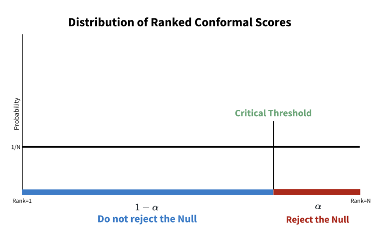
- x-axis corresponds to an ordered set of conformity scores
- If \(\alpha = 0.05\), find the score value at the the 95th percentile (e.g.
quantile(scores, 0.95)) - Blue: conformity scores are not statistically significant. They’re within our prediction interval.
- Red: Very large conformity scores indicate high divergence from the true label. These conformal scores are statistically significant and thereby outside of our prediction interval.
- Predict on the Test set and calculate conformity scores for each class
- For each test set observation, select classes that have scores below the threshold score as the model prediction.
- An observation could potentially have both classes or no classes selected. ( Not sure if this is true in a binary outcome situation)
- Example: LAC Method, Multinomial
Model
classifier = LogisticRegression(random_state=42)
classifier.fit(X_train, y_train)
Scores calculated using only the predicted probability for the true class on the Validation set (aka Calibration set)
# Get predicted probabilities for calibration set
y_pred = classifier.predict(X_Cal)
y_pred_proba = classifier.predict_proba(X_Cal)
si_scores = []
# Loop through all calibration instances
for i, true_class in enumerate(y_cal):
    # Get predicted probability for observed/true class
    predicted_prob = y_pred_proba[i][true_class]
    si_scores.append(1 - predicted_prob)
The threshold determines what coverage our predicted labels will have
number_of_samples = len(X_Cal) alpha = 0.05 qlevel = (1 - alpha) * ((number_of_samples + 1) / number_of_samples) threshold = np.percentile(si_scores, qlevel*100) print(f'Threshold: {threshold:0.3f}') #> Threshold: 0.598- Finite sample correction for the 95th quantile: multiply 0.95 by (n+1)/n
Threshold is then used to get predicted labels of the test set
# Get standard predictions for comparison y_pred = classifier.predict(X_test) # Calc scores, then only take scores in the 95% conformal PI prediction_sets = (1 - classifier.predict_proba(X_test) <= threshold) # Get labels for predictions in conformal PI def get_prediction_set_labels(prediction_set, class_labels): # Get set of class labels for each instance in prediction sets prediction_set_labels = [ set([class_labels[i] for i, x in enumerate(prediction_set) if x]) for prediction_set in prediction_sets] return prediction_set_labels # Compare conformal prediction with observed and traditional preds results_sets = pd.DataFrame() results_sets['observed'] = [class_labels[i] for i in y_test] results_sets['conformal'] = get_prediction_set_labels(prediction_sets, class_labels) results_sets['traditional'] = [class_labels[i] for i in y_pred] results_sets.head(10) #> observed conformal traditional #> 0 blue {blue} blue #> 1 green {green} green #> 2 blue {blue} blue #> 3 green {green} green #> 4 orange {orange} orange #> 5 orange {orange} orange #> 6 orange {orange} orange #> 7 orange {blue, orange} blue #> 8 orange {orange} orange #> 9 orange {orange} orange- conformity scores are calculated for each potential class using the predicted probabilities on the test set
- The predicted class for an observation is determined by whether a class has a score below the threshold.
- Therefore, an observation may have 1 or more predicted classes or 0 predicted classes.
Statistics (See Statistics section for functions)
Overall
weighted_coverage = get_weighted_coverage( results['Coverage'], results['Class counts']) weighted_set_size = get_weighted_set_size( results['Average set size'], results['Class counts']) print (f'Overall coverage: {weighted_coverage}') print (f'Average set size: {weighted_set_size}') #> Overall coverage: 0.947 #> Average set size: 1.035- Overall coverage is very close to the target coverage of 95%, therefore, marginal coverage is achieved which is expected for this method
Per Class
results = pd.DataFrame(index=class_labels) results['Class counts'] = get_class_counts(y_test) results['Coverage'] = get_coverage_by_class(prediction_sets, y_test) results['Average set size'] = get_average_set_size(prediction_sets, y_test) results #> Class counts Coverage Average set size #> blue 241 0.817427 1.087137 #> orange 848 0.954009 1.037736 #> green 828 0.977053 1.016908- Overall coverage (i.e. for all labels) will be at or very near 95% but coverage for individual classes may vary.
- An illustration of how this method lacks Conditional Coverage
- Solution: Get thresholds for each class. (See next example)
- Note that the blue class had substantially fewer observations that the other 2 classes.
- Overall coverage (i.e. for all labels) will be at or very near 95% but coverage for individual classes may vary.
- Example: LAC-adapted - Threshold per Class
Don’t think {{mapie}} has this option.
Also possible do this for subgroups of data, such as ensuring equal coverage for a diagnostic across racial groups, if we found coverage using a shared threshold led to problems.
Calculate individual class thresholds
# Set alpha (1 - coverage)
alpha = 0.05
thresholds = []
# Get predicted probabilities for calibration set
y_cal_prob = classifier.predict_proba(X_Cal)
# Get 95th percentile score for each class's s-scores
for class_label in range(n_classes):
    mask = y_cal == class_label
    y_cal_prob_class = y_cal_prob[mask][:, class_label]
    s_scores = 1 - y_cal_prob_class
    q = (1 - alpha) * 100
    class_size = mask.sum()
    correction = (class_size + 1) / class_size
    q *= correction
    threshold = np.percentile(s_scores, q)
    thresholds.append(threshold)
Apply individual class thresholds to test set scores
# Get Si scores for test set
predicted_proba = classifier.predict_proba(X_test)
si_scores = 1 - predicted_proba

# For each class, check whether each instance is below the threshold
prediction_sets = []
for i in range(n_classes):
    prediction_sets.append(si_scores[:, i] <= thresholds[i])
prediction_sets = np.array(prediction_sets).T

# Get prediction set labels and show first 10
prediction_set_labels = get_prediction_set_labels(prediction_sets, class_labels)
Statistics
Overall
weighted_coverage = get_weighted_coverage( results['Coverage'], results['Class counts']) weighted_set_size = get_weighted_set_size( results['Average set size'], results['Class counts']) print (f'Overall coverage: {weighted_coverage}') print (f'Average set size: {weighted_set_size}') #> Overall coverage: 0.95 #> Average set size: 1.093- Similar to previous example
Per Class
results = pd.DataFrame(index=class_labels) results['Class counts'] = get_class_counts(y_test) results['Coverage'] = get_coverage_by_class(prediction_sets, y_test) results['Average set size'] = get_average_set_size(prediction_sets, y_test) results #> Class counts Coverage Average set size #> blue 241 0.954357 1.228216 #> orange 848 0.956368 1.139151 #> green 828 0.942029 1.006039- Coverages now very close to 95% and the average set sizes have increased, especially for Blue.
Continuous
Conformalized Quantile Regression Process
- Split data into Training, Calibration, and Test sets
- Training data: data on which the quantile regression model learns.
- Calibration data: data on which CQR calibrates the intervals.
- In the example, he split the data into 3 equal sets
- Test data: data on which we evaluate the goodness of intervals.
- Fit quantile regression model on training data.
- Use the model obtained at previous step to predict intervals on calibration data.
- PIs are predictions at the quantiles:
- (alpha/2)*100) (e.g 0.025, alpha = 0. 05)
- (1-(alpha/2))*100) (e.g. 0.975)
- PIs are predictions at the quantiles:
- Compute conformity scores on calibration data and intervals obtained at the previous step.
- Residuals are calculated for the PI vectors
- Scores are calculated by taking the row-wise maximum of both (upper/lower quantile) residual vectors (e.g
s_i <- pmax(lower_pi_res, upper_pi_res))
- Get 1-alpha quantile from the distribution of conformity scores (e.g
threshold <- quantile(s_i, 0.95)- This score value will be the threshold
- Use the model obtained at step 1 to make predictions on test data.
- Compute PI vectors (i.e. predictions at the previously stated quantiles) on Test set
- i.e. Same calculation as with the calibration data in step 2 where you use the model to predict at upper and lower PI quantiles.
- Compute lower/upper end of the interval by subtracting/adding the threshold from/to the quantile predictions (aka PIs)
- Lower conformity interval:
lower_pi <- test_lower_pred - threshold - Upper conformity interval:
upper_pi <- test_upper_pred + threshold
- Lower conformity interval:
- Split data into Training, Calibration, and Test sets
Example: Quantile Random Forest
import numpy as np
from skgarden import RandomForestQuantileRegressor

alpha = .05

# 1. Fit quantile regression model on training data
model = RandomForestQuantileRegressor().fit(X_train, y_train)

# 2. Make prediction on calibration data
y_cal_interval_pred = np.column_stack([
    model.predict(X_cal, quantile=(alpha/2)*100),
    model.predict(X_cal, quantile=(1-alpha/2)*100)])

# 3. Compute conformity scores on calibration data
y_cal_conformity_scores = np.maximum(
    y_cal_interval_pred[:,0] - y_cal,
    y_cal - y_cal_interval_pred[:,1])

# 4. Threshold: Get 1-alpha quantile from the distribution of conformity scores
#    Note: this is a single number
quantile_conformity_scores = np.quantile(
    y_cal_conformity_scores, 1-alpha)

# 5. Make prediction on test data
y_test_interval_pred = np.column_stack([
    model.predict(X_test, quantile=(alpha/2)*100),
    model.predict(X_test, quantile=(1-alpha/2)*100)])

# 6. Compute left (right) end of the interval by
#    subtracting (adding) the quantile to the predictions
y_test_interval_pred_cqr = np.column_stack([
    y_test_interval_pred[:,0] - quantile_conformity_scores,
    y_test_interval_pred[:,1] + quantile_conformity_scores])
Statistics
- Average Set Size
The average number of predicted classes per observation since there can be more than 1 predicted class in the conformal PI
Example:
# average set size for each class
def get_average_set_size(prediction_sets, y_test):
    average_set_size = []
    for i in range(n_classes):
        average_set_size.append(
            np.mean(np.sum(prediction_sets[y_test == i], axis=1)))
    return average_set_size

# Overall average set size (weighted by class size)
# Get class counts
def get_class_counts(y_test):
    class_counts = []
    for i in range(n_classes):
        class_counts.append(np.sum(y_test == i))
    return class_counts

def get_weighted_set_size(set_size, class_counts):
    total_counts = np.sum(class_counts)
    weighted_set_size = np.sum((set_size * class_counts) / total_counts)
    weighted_set_size = round(weighted_set_size, 3)
    return weighted_set_size
- Coverage
Classification: Percentage of correct classifications
Example: Classification
# coverage for each class
def get_coverage_by_class(prediction_sets, y_test):
    coverage = []
    for i in range(n_classes):
        coverage.append(np.mean(prediction_sets[y_test == i, i]))
    return coverage

# overall coverage (weighted by class size)
# Get class counts
def get_class_counts(y_test):
    class_counts = []
    for i in range(n_classes):
        class_counts.append(np.sum(y_test == i))
    return class_counts

def get_weighted_coverage(coverage, class_counts):
    total_counts = np.sum(class_counts)
    weighted_coverage = np.sum((coverage * class_counts) / total_counts)
    weighted_coverage = round(weighted_coverage, 3)
    return weighted_coverage
Visualization
- Confusion Matrix
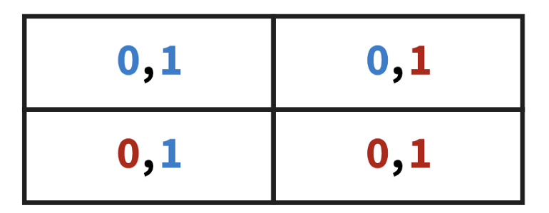
- Binary target where labels are 0 and 1
- Interpretation
- Top-left: predictions where both labels are not statistically significant (i.e. inside the “prediction interval”).
- The model predicts both classes well since both labels have low scores.
- Depending the threshold, maybe the model could be relatively agnostic (e.g. predicted probabilites like 0.50-0.50, 0.60-0.40)
- Bottom-right: predictions where both labels are statistically significant (i.e. outside the “prediction interval”).
- Model totally whiffs. Confident it’s one label when it’s actually another.
- Example
- 1 (truth) - low predicted probability = high score -> Red and significant
- 0 - high predicted probability = high score -> Red and significant
- Example
- Model totally whiffs. Confident it’s one label when it’s actually another.
- Top-right: predictions where all 0 labels are not statistically significant.
- Model predicted the 0=class well (i.e. low scores) but the 1-class poorly (i.e. high scores)
- Bottom-left: predictions where all 1 labels are not statistically significant. Here, the model predicted that 1 is the true class.
- Vice versa of top-right
- Top-left: predictions where both labels are not statistically significant (i.e. inside the “prediction interval”).