LaTeX

Misc

The pound sign (#) must be escaped with a backslash (\) in the code. Otherwise the latex won’t be rendered in the html document.

Examples

R = 
\begin{pmatrix}
1 & r_0r & r_0r^2 & \cdots & r_0r^{T-1} \\
r_0r & 1 & r_0r & \cdots & r_0r^{T-2} \\
r_0r^2 & r_0r & 1 & \cdots & r_0r^{T-3} \\ 
\vdots & \vdots & \vdots & \vdots & \vdots \\ 
r_0r^{T-1} & r_0r^{T-2} & r_0r^{T-3} & \cdots & 1 
\end{pmatrix}

\[ R = \begin{pmatrix} 1 & r_0r & r_0r^2 & \cdots & r_0r^{T-1} \\ r_0r & 1 & r_0r & \cdots & r_0r^{T-2} \\ r_0r^2 & r_0r & 1 & \cdots & r_0r^{T-3} \\ \vdots & \vdots & \vdots & \vdots & \vdots \\ r_0r^{T-1} & r_0r^{T-2} & r_0r^{T-3} & \cdots & 1 \end{pmatrix} \]

s(\\boldsymbol{\\hat{\\theta}}, y) = 
\begin{pmatrix} 
s(\hat{\theta}, y_1)_1 & s(\hat{\theta}, y_1)_2 & \cdots & s(\hat{\theta}, y_1)_k \\
\vdots & \vdots & \ddots & \vdots \\
s(\hat{\theta}, y_n)_1 & s(\hat{\theta}, y_n)_2 & \cdots & s(\hat{\theta}, y_n)_k \\
\end{pmatrix}

\[ s(\boldsymbol{\hat{\theta}}, y) = \begin{pmatrix} s(\hat{\theta}, y_1)_1 & s(\hat{\theta}, y_1)_2 & \cdots & s(\hat{\theta}, y_1)_k \\ \vdots & \vdots & \ddots & \vdots \\ s(\hat{\theta}, y_n)_1 & s(\hat{\theta}, y_n)_2 & \cdots & s(\hat{\theta}, y_n)_k \\ \end{pmatrix} \]

[1 \; x_{1t} \; x_{2t} \; \cdots \; x_{mt}] 
\cdot \left( \begin{array}{ccc} 
\hat{\beta}_{01} & \cdots & \hat{\beta}_{0k} \\ 
\vdots & \ddots & \vdots \\ 
\hat{\beta}_{m1} & \cdots & \hat{\beta}_{mk} \end{array} \right) 
= 
[\hat{y}_{t1} \; \hat{y}_{t2} \; \cdots \; \hat{y}_{tk}]

\[ [1 \; x_{1t} \; x_{2t} \; \cdots \; x_{mt}] \cdot \left( \begin{array}{ccc} \hat{\beta}_{01} & \cdots & \hat{\beta}_{0k} \\ \vdots & \ddots & \vdots \\ \hat{\beta}_{m1} & \cdots & \hat{\beta}_{mk} \end{array} \right) = [\hat{y}_{t1} \; \hat{y}_{t2} \; \cdots \; \hat{y}_{tk}] \]

ICC_{tt} = ICC_{tt'} = \frac {\sigma_b^2} {\sigma_b^2 + \sigma_e^2} r_{tt'}

\[ ICC_{tt} = ICC_{tt'} = \frac {\sigma_b^2} {\sigma_b^2 + \sigma_e^2} r_{tt'} \]

y_{ict} = \mu + \beta_0t + \beta_1X_{ct} + b_{ct} + e_{ict}

\[ y_{ict} = \mu + \beta_0t + \beta_1X_{ct} + b_{ct} + e_{ict} \]

\hat{\theta} = \arg\max_{\theta \in \Theta} \sum\_{i=1}^n w_i^{\text{forest}} \\cdot l(\theta; y_i)

\[ \hat{\theta} = \arg\max_{\theta \in \Theta} \sum_{i=1}^n w_i^{\text{forest}} \cdot l(\theta; y_i) \]

\begin{align*}
H(Y|X_1,\cdots, X_k) = \sum_{d = 0,1} \sum_{{i_1}=1}^c \cdots \sum_{{i_k}=1}^c \\
P(y_d | x_{i_1}, \cdots, x_{i_k}) \log P(y_d | x_{i_1}, \cdots, x_{i_k})
\end{align*}

\[ \begin{align*} H(Y|X_1,\cdots, X_k) = \sum_{d = 0,1} \sum_{{i_1}=1}^c \cdots \sum_{{i_k}=1}^c \\ P(y_d | x_{i_1}, \cdots, x_{i_k}) \log P(y_d | x_{i_1}, \cdots, x_{i_k}) \end{align*} \]

\begin{align*}
x^2 + y^2 &= 1 \\
y &= \sqrt{1 - x^2}
\end{align*}

With the “&” symbols, the 2nd line stays lined up with the end of the first line

\[ \begin{align*} x^2 + y^2 &= 1 \\ y &= \sqrt{1 - x^2} \end{align*} \]

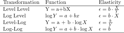
\begin{tabular} {lll}
Transformation & Function & Elasticity \\
\hline
Level Level & Y\;=\;a+bX & \epsilon = b \cdot \frac {X} {Y} \\  
Log Level & \log Y = a+bx & \epsilon = b \cdot X \\
Level-Log & Y = a + b \cdot \log X & \epsilon = \frac {b} {Y} \\
Log-Log & \log Y = a + b \cdot \log X & \epsilon = b \\
\hline
\end{tabular}

This is “Raw LaTeX” and will be ignored when the output is HTML. (See Docs)
In the last column, for some unknown reason, using \frac without another “\” symbol before it throws an error. Adding \epsilon = to the expression made it work fine.

c_{max}(t,\mu, \sigma) = \max \limits_{k = 1,..., dim(T)} \left | \frac {(t-\mu)_k} {\sqrt {\Sigma_{kk}}} \right |

Large absolute pipes require \left, \right
The text underneath “max” requires \limits

\[ c_{max}(t,\mu, \sigma) = \max \limits_{k = 1,..., dim(T)} \left | \frac {(t-\mu)_k} {\sqrt {\Sigma_{kk}}} \right | \]

\begin{align*}
\mbox{net present value (npv)} = &\sum \limits_{i = 0}^m benefit_i*(1-discount)^i -\\
&\sum \limits_{i=0}^m cost_i*(1-discount)^i
\end{align*}

\[ \begin{align*} \mbox{net present value (npv)} = &\sum \limits_{i = 0}^m benefit_i*(1-discount)^i -\\ &\sum \limits_{i=0}^m cost_i*(1-discount)^i \end{align*} \]

\epsilon_Z \stackrel{\text{iid}}{\sim} \mathcal{N}(0, 0.1)

\[ \epsilon_Z \stackrel{\text{iid}}{\sim} \mathcal{N}(0, 0.1) \]

\mbox{posterior} = \frac {\mbox{Prob of observed variables} \;\times\; \mbox{Prior}} {\mbox{Normalizing constant}}

\[ \mbox{posterior} = \frac {\mbox{Prob of observed variables} \;\times\; \mbox{Prior}} {\mbox{Normalizing constant}} \]

\lim\limits_{x \to +\infty} \sup \frac{\bar{F}(x)}{\bar{F}_{\exp}(x)} = \frac{\bar{F}(x)}{e^{-\lambda x}}, \;\; \forall \lambda > 0

\[ \lim\limits_{x \to +\infty} \sup \frac{\bar{F}(x)}{\bar{F}_{\exp}(x)} = \frac{\bar{F}(x)}{e^{-\lambda x}}, \;\; \forall \lambda > 0 \]

\text{vec} = \left( \begin{array}{cc} \text{rand var1} \\
 \text {rand var2} \end{array} \right)

\[ \text{vec} = \left( \begin{array}{cc} \text{rand var1} \\ \text {rand var2} \end{array} \right) \]

SBD(x,y) = 1 - \frac {\max (\text{NCCc}(x,y))} {\left\lVert x \right\rVert_2 \; \left\lVert y \right\rVert_2}

\[ SBD(x,y) = 1 - \frac {\max (\text{NCCc}(x,y))} {\left\lVert x \right\rVert_2 \; \left\lVert y \right\rVert_2} \]

\begin{align}
&D \not\!\perp\!\!\!\perp A \\
&D \!\perp\!\!\!\perp A \\
&Y \!\perp\!\!\!\perp X|Z
&Y \perp\mkern-10mu\perp X\;|\;Z
\end{align}

\[ \begin{align} &D \not\!\perp\!\!\!\perp A \\ &D \!\perp\!\!\!\perp A \\ &Y \!\perp\!\!\!\perp X|Z \\ &Y \perp\mkern-10mu\perp X\;|\;Z \end{align} \]

||y-f||^2 + \lambda \int \left(\frac {\partial^2 f(\text{log[baseline profit]})}{\partial \; \text{log[baseline profit]}^2}\right)^2 \partial x

\[ ||y-f||^2 + \lambda \int \left(\frac {\partial^2 f(\text{log[baseline profit]})}{\partial \; \text{log[baseline profit]}^2}\right)^2 \partial x \]

E_{iz_{nm}} = 
\left\{ \begin{array}{lcl}
-\beta_z z_{zm}P_{nm} \left(1+ \frac{1-\lambda_k}{\lambda_k} \frac {1}{P_{nB_k}} \right) & \mbox{if} \; m \in \beta_k \\
-\beta_z z_{zm}P_{nm} & \mbox{if} \; m \in \beta_k 
\end{array}\right.

There is no dash between {array} and {lcl}. It’s just two curly brackets touching each other
- If you want the expressions on the left side to right-align use {rcl} — for center-align, leave it blank I think
Do not forget that period at end — to the right of \right

\[ E_{iz_{nm}} = \left\{ \begin{array}{lcl} -\beta_z z_{zm}P_{nm} \left(1+ \frac{1-\lambda_k}{\lambda_k} \frac {1}{P_{nB_k}} \right) & \mbox{if} \; m \in \beta_k \\ -\beta_z z_{zm}P_{nm} & \mbox{if} \; m \notin \beta_k \end{array}\right. \]

\begin{align}
&P_{ni} = \int L_{ni}(\beta) \; f(\beta\;|\;\boldsymbol{\theta}) d\beta\\
&\mbox{where} \; L_{ni}(\beta) = \frac {e^{V_{ni}(\beta)}}{\sum_{j=1}^J e^{V_{ni}(\beta)}} 
\end{align}

Alignment occurs where the & symbols are positioned
\boldsymbol is used bold the vector \(\theta\)

\[ \begin{align} &P_{ni} = \int L_{ni}(\beta) \; f(\beta\;|\;\boldsymbol{\theta}) \; d\beta\\ &\mbox{where} \; L_{ni}(\beta) = \frac {e^{V_{ni}(\beta)}}{\sum_{j=1}^J e^{V_{ni}(\beta)}} \end{align} \]

\pi_i = \mbox{Pr}(i \in S) = \sum \limits_{i \in s \in S} \mbox{Pr}(S = s) = \frac {\binom{N-1}{n-1}}{\binom{N}{n}} = \frac {n}{N}

\binom used for binomial coefficient/combination notation

\[ \pi_i = \mbox{Pr}(i \in S) = \sum \limits_{i \in s \in S} \mbox{Pr}(S = s) = \frac {\binom{N-1}{n-1}}{\binom{N}{n}} = \frac {n}{N} \]

\begin{aligned}
&R_{i,j} = \frac{S_i + S_j}{M_{i,j}}\\
&\begin{aligned}
\text{where} \;\; &S_i = \left(\frac{1}{T_i} \sum_{j=1}^{T_i} \lVert X_j - A_i \rVert_{p}^q \right)^{\frac{1}{q}} \;\; \text{and} \\
&M_{i,j} = \lVert A_i - A_j \rVert_p = \left(\sum_{k=1}^n |a_{k,i} - a_{k,j}|^p\right)^{\frac{1}{p}}
\end{aligned}
\end{aligned}

The key for this nested align is the “&” before the second \begin{aligned}. Otherwise “where” and \(R_{i,j}\) won’t be aligned flushly on the left side.

\[ \begin{aligned} &R_{i,j} = \frac{S_i + S_j}{M_{i,j}}\\ &\begin{aligned} \text{where} \;\; &S_i = \left(\frac{1}{T_i} \sum_{j=1}^{T_i} \lVert X_j - A_i \rVert_{p}^q \right)^{\frac{1}{q}} \;\; \text{and} \\ &M_{i,j} = \lVert A_i - A_j \rVert_p = \left(\sum_{k=1}^n |a_{k,i} - a_{k,j}|^p\right)^{\frac{1}{p}} \end{aligned} \end{aligned} \]

\begin{aligned}
&Y_{ij} = [\alpha_0 + \beta_0 \text{large}_{ij}] + [u_i + v_i \text{large}_{ij} + \epsilon_{ij}] \\
&\begin{aligned}
\text{where}\quad \epsilon &\sim \mathcal{N}(0, \sigma^2) \: \text{and}\\
\left[ \begin{array}{cc} u_i \\ v_i \end{array} \right] &\sim \mathcal{N} \left(\left[\begin{array}{cc} 0\\0 \end{array}\right], \left[\begin{array}{cc} \sigma^2_u\\\rho\sigma_u \sigma_v \quad \sigma^2_v \end{array}\right]\right)
\end{aligned}
\end{aligned}

\[ \begin{aligned} &Y_{ij} = [\alpha_0 + \beta_0 \text{large}_{ij}] + [u_i + v_i \text{large}_{ij} + \epsilon_{ij}] \\ &\begin{aligned} \text{where}\quad \epsilon &\sim \mathcal{N}(0, \sigma^2) \: \text{and}\\ \left[ \begin{array}{cc} u_i \\ v_i \end{array} \right] &\sim \mathcal{N} \left(\left[\begin{array}{cc} 0\\0 \end{array}\right], \left[\begin{array}{cc} \sigma^2_u\\\rho\sigma_u \sigma_v \quad \sigma^2_v \end{array}\right]\right) \end{aligned} \end{aligned} \]

\left[\begin{array}{cc} u_i\\v_i\\w_i\\x_i\\y_i\\z_i \end{array} \right] 
\sim \mathcal{N} \left(
\left[\begin{array}{cc} 0\\0\\0\\0\\0\\0\end{array} \right],
\begin{bmatrix}
\sigma_u^2 \\
\sigma_{uv} & \sigma_v^2 \\
\sigma_{uw} & \sigma_{vw} & \sigma^2_w \\
\sigma_{ux} & \sigma_{vx} & \sigma_{wx} & \sigma_x^2 \\
\sigma_{uy} & \sigma_{vy} & \sigma_{wy} & \sigma_{xy} & \sigma_{y}^2 \\
\sigma_{uz} & \sigma_{vz} & \sigma_{wz} & \sigma_{xz} & \sigma_{yz} & \sigma_z^2
\end{bmatrix}
\right)

bmatrix stands for bracket matrix. Previous matrices (above) used pmatrix which stands for parentheses matrix.
Others:
- Bmatrix for curly braces matrix
- vmatrix for a matrix with “rectangular line boundary”
- Vmatrix for a matrix with double vertical bars
- matrix for a matrix without brackets

\[ \left[\begin{array}{cc} u_i\\v_i\\w_i\\x_i\\y_i\\z_i \end{array} \right] \sim \mathcal{N} \left( \left[\begin{array}{cc} 0\\0\\0\\0\\0\\0\end{array} \right], \begin{bmatrix} \sigma_u^2 \\ \sigma_{uv} & \sigma_v^2 \\ \sigma_{uw} & \sigma_{vw} & \sigma^2_w \\ \sigma_{ux} & \sigma_{vx} & \sigma_{wx} & \sigma_x^2 \\ \sigma_{uy} & \sigma_{vy} & \sigma_{wy} & \sigma_{xy} & \sigma_{y}^2 \\ \sigma_{uz} & \sigma_{vz} & \sigma_{wz} & \sigma_{xz} & \sigma_{yz} & \sigma_z^2 \end{bmatrix} \right) \]

\begin{align}
&\ \textbf{Registered provinces for INGO } i \\
\text{Count of provinces}\ \sim&\ \operatorname{Ordered\,Beta}(\mu_{i_j}, \phi_y, k_{0_y}, k_{1_y}) \\[8pt]
&\textbf{Model of Outcome Average} \\
\mu_i = &\
  \mathrlap{\begin{aligned}[t]
  &\beta_0 + \beta_1\ \text{Issue[Arts and Culture]} + \beta_2\ \text{Issue[Education]}\ + \\
  &\beta_3\ \text{Issue[Industry and Humanitarian]} + \beta_4\ \text{Issue[Economy and Trade]}
  \end{aligned}}\\[8pt]
&\ \textbf{Priors} \\
\beta_0\ \sim&\ \operatorname{Student\,t}(\nu = 3, \mu = 0, \sigma = 2.5) && \text{Intercept} \\
\beta_{1..12}\ \sim&\ \mathcal{N}(0, 5) && \text{Coefficients}
\end{align}

textbf is bold font text
\operatorname treats text as functions like \max or \sin in terms of spacing
\mathrlap + \begin{aligned}allows you to wrap extra long equations

\[ \begin{align} &\ \textbf{Registered Provinces for INGO } i \\ \text{Count of Provinces}\ \sim&\ \operatorname{Ordered\,Beta}(\mu_{i_j}, \phi_y, k_{0_y}, k_{1_y}) \\[8pt] &\textbf{Model of Outcome Average} \\ \mu_i = &\ \mathrlap{\begin{aligned}[t] &\beta_0 + \beta_1\ \text{Issue[Arts and Culture]} + \beta_2\ \text{Issue[Education]}\ + \\ &\beta_3\ \text{Issue[Industry and Humanitarian]} + \beta_4\ \text{Issue[Economy and Trade]} \end{aligned}}\\[4pt] &\ \textbf{Priors} \\ \beta_0\ \sim&\ \operatorname{Student\,t}(\nu = 3, \mu = 0, \sigma = 2.5) && \text{Intercept} \\ \beta_{1..12}\ \sim&\ \mathcal{N}(0, 5) && \text{Coefficients} \end{align} \]

\begin{align}
  \text{Transition}_{\text{2-step}} &= 
  \begin{aligned}[t]
    &P(X_{n-1} = 0|X_{n-2} = 0) \cdot P(X_n = 1|X_{n-1} = 0) \\
    &+ P(X_{n-1} = 1|X_{n-2} = 0) \cdot P(X_n = 1|X_{n-1} = 1) \\
    &+ P(X_{n-1} = 2|X_{n-2} = 0) \cdot P(X_n = 1|X_{n-1} = 2)
  \end{aligned}\\
  &= (0.7 \cdot 0.2) + (0.3 \cdot 0.4) + (0 \cdot 0) = 0.33
\end{align}

[t] says this nested aligned section should be top aligned with “Transition” and not centered on “Transition.”

\[ \begin{align} \text{Transition}_{\text{2-step}} &= \begin{aligned}[t] &P(X_{n-1} = 0|X_{n-2} = 0) \cdot P(X_n = 1|X_{n-1} = 0) \\ &+ P(X_{n-1} = 1|X_{n-2} = 0) \cdot P(X_n = 1|X_{n-1} = 1) \\ &+ P(X_{n-1} = 2|X_{n-2} = 0) \cdot P(X_n = 1|X_{n-1} = 2) \end{aligned}\\ &= (0.7 \cdot 0.2) + (0.3 \cdot 0.4) + (0 \cdot 0) = 0.33 \end{align} \]

\underbrace{\frac{P(M_1|D)}{P(M_2|D)}}_{\text{Posterior Odds}} = 
\underbrace{\frac{P(D|M_1)}{P(D|M_2)}}_{\text{Likelihood Ratio}} 
\times
\underbrace{\frac{P(M_1)}{P(M_2)}}_{\text{Prior Odds}}

\[ \underbrace{\frac{P(M_1|D)}{P(M_2|D)}}_{\text{Posterior Odds}} = \underbrace{\frac{P(D|M_1)}{P(D|M_2)}}_{\text{Likelihood Ratio}} \times \underbrace{\frac{P(M_1)}{P(M_2)}}_{\text{Prior Odds}} \]

\begin{array}{c|cccc}
& A & B & C & D \\
\hline
A & 0 & 0.66 & 0.34 & 0 \\
B & 0.50 & 0 & 0.50 & 0 \\
C & 0 & 0.61 & 0 & 0.39 \\
D & 0 & 0.28 & 0.72 & 0
\end{array}

\[ \begin{array}{c|cccc} & A & B & C & D \\ \hline A & 0 & 0.66 & 0.34 & 0 \\ B & 0.50 & 0 & 0.50 & 0 \\ C & 0 & 0.61 & 0 & 0.39 \\ D & 0 & 0.28 & 0.72 & 0 \end{array} \]