MLOps
Misc
- {collateral} - Captures side effects like errors to prevent them from stopping execution. Once your analysis is done, you can see a tidy view of the groups that failed, the ones that returned a results, and the ones that threw warnings, messages or other output as they ran.
- {config} - Makes it easy to manage environment specific configuration values.
- {frontmatter} - Extracts and parses structured metadata (‘YAML’ or ‘TOML’) from the beginning of text documents. (Uses {tomledit}, {yaml12})
- {onnx} - ‘ONNX’ provides an open source format for machine learning models through {reticulate}
- {onnxr} - Directly interfaces with ONNX runtime’s C++ API via cpp11. This uses far less memory and does not require a Python and TensorFlow installation.
- {PyMilo} (JOSS) - Serializes models in a transparent human-readable format (e.g. JSON) that preserves end-to-end model fidelity and enables reliable, safe, and interpretable exchange
- {ryl} (vs code ext, github) - Rust-based YAML linter
- {S7schema} - ‘S7’ Framework for Schema-Validated YAML Configuration. Validates YAML through a json schema file.
- {strata} - Simple project automation framework
- Supports {renv}, {cronR}, and {taskscheduleR}
- Simple and consistent built-in logging
- Manage code execution in
.tomlfiles - Quick build options for rapid prototyping
- {yaml12}, {yaml12} - Fast, correct, and safe YAML 1.2 parsing and emitting, built in Rust.
- Tools
- Ray
- Weights and Biases - Experiment tracking for Python
- Monitoring Dashboard
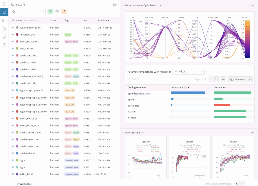
- Allows you to compare the results of different experiments, the hyperparameters used, and the training curves. It also tracks system metrics such as GPU and CPU usage.
- Integrates with Huggingface
- Free Tier (Paid tier also includes notification, team collaboration, CI/CD)
- AI application evaluations
- AI application tracing
- AI application scorers
- AI model experiment tracking
- AI assets registry & lineage tracking
- Community Support
- Supports Hydra - YAML config system for experimentation (How to use Hydra with W&B)
- Monitoring Dashboard
- Resources
- Python model storage formats and their issues
- Notes from {PyMilo} JOSS
- Pickle
- Loading a pickle file may execute arbitrary code contained within it, a known vulnerability that can be exploited if the file is maliciously crafted. Serialized files are opaque binary blobs that cannot be inspected without loading
- Pickle files often depend on specific library versions, which may hinder long-term reproducibility.
- Open Neural Network Exchange (ONNX) and Predictive Model Markup Language (PMML) convert trained models into framework agnostic representations.
- ONNX uses a graph-based structure built from primitive operators (e.g., linear transforms, activations), while PMML provides an XML-based specification for traditional models like decision trees and regressions
- Exporting complex pipelines to ONNX or PMML often leads to structural approximations, missing metadata, or unsupported components, especially for customized models. As a result, the exported model may differ in behavior, resulting in performance degradation or loss of accuracy
- ONNX uses a binary protocol buffer format that is not human-readable, which limits interpretability and makes auditing difficult. PMML, although XML-based and readable, is verbose and narrowly scoped, supporting only a limited subset of scikit-learn models
- PMML does not provide a mechanism to restore exported models into Python, making it a one-way format that limits reproducibility across ML workflows
- SKOPS improves the safety of scikit-learn model storage by enabling limited inspection of model internals without requiring code execution.
- Only supports scikit-learn models, lacks compatibility with other frameworks, and does not provide a fully transparent or human-readable structure.
- TensorFlow.js converts TensorFlow or Keras models into a JSON configuration file and binary weight files for execution in the browser or Node.js
- Has been shown to introduce compatibility issues, performance degradation, and inconsistencies in inference behavior due to backend limitations and environment-specific faults.
- Models from other frameworks, such as scikit-learn or PyTorch, must be re-implemented or retrained in TensorFlow to be exported.
- Running complex models in JavaScript runtimes introduces memory and performance limitations, often making the deployment of large neural networks prohibitively slow or even infeasible in browser environments
- Logging
Also see R >> Code >> mlops >> manual-logging.R for more details/use cases
Example: Manual Logging (source)
Code
OUTPUT_DIR <- "reports" # Create output directory if (!dir.exists(OUTPUT_DIR)) { dir.create(OUTPUT_DIR, recursive = TRUE) cat(sprintf("Created output directory: %s\n", OUTPUT_DIR)) } # Initialize logging log_file <- file.path( OUTPUT_DIR, sprintf("burst-report-log_%s.txt", format(Sys.time(), "%Y%m%d_%H%M%S")) ) log_conn <- file(log_file, open = "wt") # level is the type of message (e.g. info, error) log_msg <- function(msg, level = "INFO") { timestamp <- format(Sys.time(), "%Y-%m-%d %H:%M:%S") log_line <- sprintf("[%s] %s: %s", timestamp, level, msg) cat(log_line, "\n", file = log_conn) cat(log_line, "\n") } # use cases log_msg("Starting burst report generation") log_msg(sprintf( "Found %d store-month combinations with >= %d orders", nrow(store_months), MIN_ORDERS )) # Close log file close(log_conn)- See R, Base >> Error Handling >>
tryCatch>> Example 3 for usage in logging error messages
- See R, Base >> Error Handling >>
Terms
- Asynchronous - Tasks run independently, and you don’t have to wait for them to finish.
- i.e. in a separate process (e.g. R process) which self-contained and only has access to data present there.
- Promise (or Future)- Represents a future value or the result of an asynchronous operation. It’s a way to handle tasks that take time to complete (e.g., fetching data, running computations, or executing code in parallel) without blocking the main program.
- i.e. an IOU/placeholder for a result that isn’t ready yet.
- Useful to:
- Avoid blocking: Instead of waiting for each task to finish, you can start all tasks at once and collect results later.
- Handle dependencies: If one task depends on the result of another, promises let you chain them together.
- Improve efficiency: By running tasks in parallel and managing their results asynchronously, you can make better use of resources.
- SSH Reverse Tunneling - Allows you to securely access a computer or server that’s behind a firewall or not directly reachable from the internet.
- Provides a convenient way to launch remote daemons without requiring the remote machine to be able to access the host. Often firewall configurations or security policies may prevent opening a port to accept outside connections.
Concepts
- Notes from
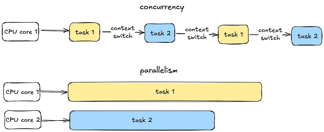
- Concurrency - Managing multiple tasks at the same time, not necessarily simultaneously. Tasks may take turns, creating the illusion of multitasking.
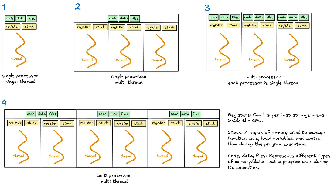
- Thread - A thread is the smallest unit of execution within a process. A process acts as a “container” for threads, and multiple threads can be created and destroyed over the process’s lifetime.
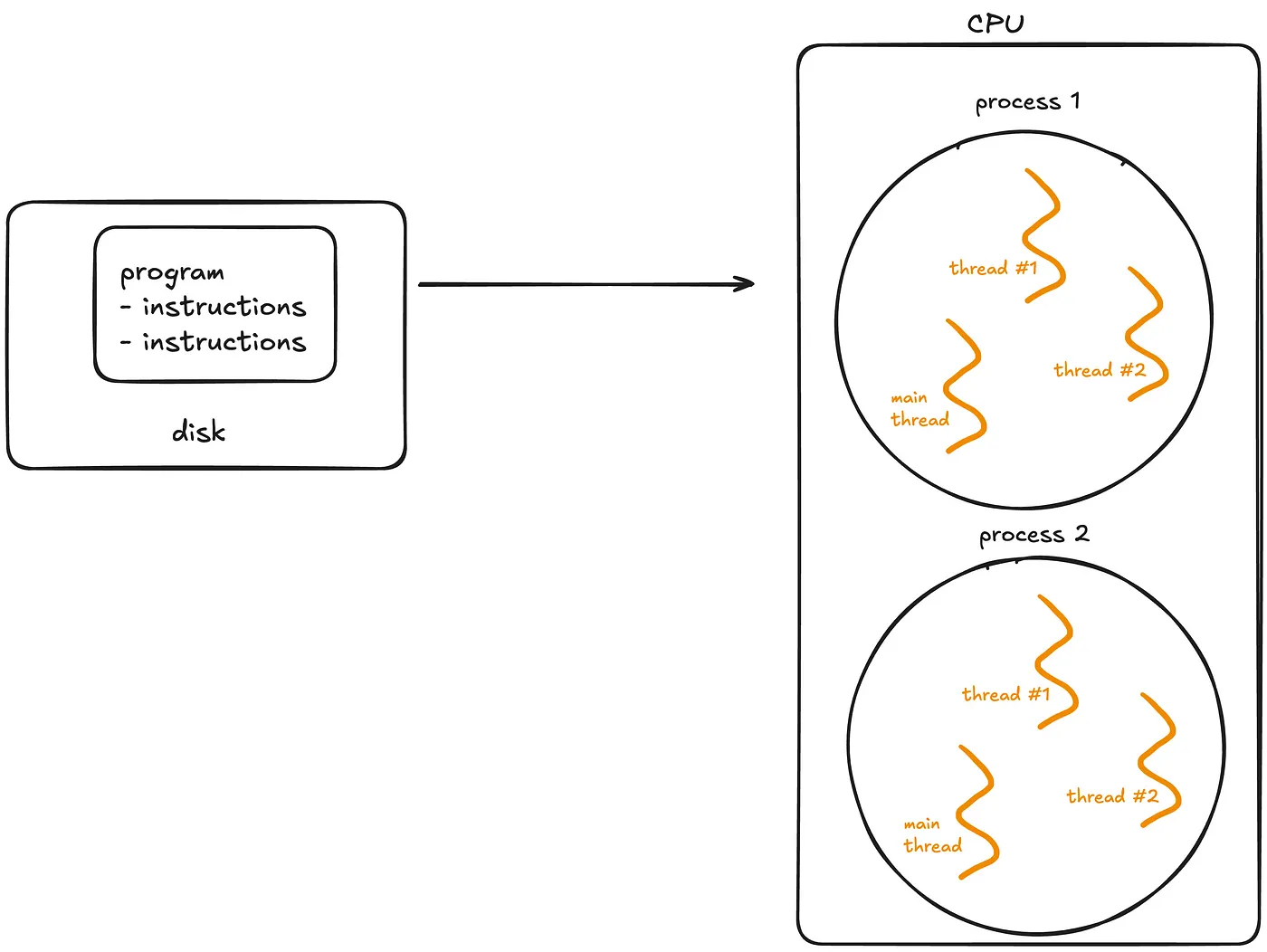
- Every process has at least one thread — the main thread — but it can also create additional threads.
- Threads share memory and resources within the same process, enabling efficient communication.
- Preemptive Context Switching - When a thread is waiting, the OS switches to another thread automatically. During a context switch, the OS pauses the current task, saves its state and loads the state of the next task to be executed. This rapid switching creates the illusion of simultaneous execution on a single CPU core.
- For processes, context switching is more resource-intensive because the OS must save and load separate memory spaces.
- For threads, switching is faster because threads share the same memory within a process.
- Multithreading - Allows a process to execute multiple threads concurrently, with threads sharing the same memory and resources.
- Global Interpreter Lock (GIL) - A lock that allows only one thread to hold control of the Python interpreter at any time, meaning only one thread can execute Python bytecode at once.
- Introduced to simplify memory management in Python as many internal operations, such as object creation, are not thread safe by default.
- Without a GIL, multiple threads trying to access the shared resources will require complex locks or synchronisation mechanisms to prevent race conditions and data corruption.
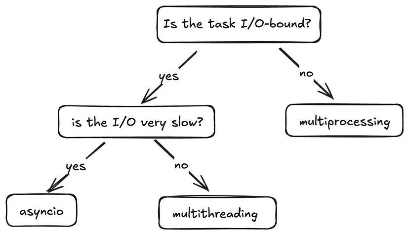
- For multithreaded I/O-bound programs, the GIL is less problematic as threads release the GIL when waiting for I/O operations.
- For multithreaded CPU-bound operations, the GIL becomes a significant bottleneck. Multiple threads competing for the GIL must take turns executing Python bytecode.
- Multiprocessing is recommended for CPU-bound tasks
- Multiprocessing - Enables a system to run multiple processes in parallel, each with its own memory, GIL, and resources. Within each process, there may be one or more threads
- Async/Await - Unlike threads or processes, async uses a single thread to handle multiple tasks.
- Differences from Multithreading
- Multithreading relies on the OS to switch between threads when one thread is waiting (preemptive context switching).
- Async/Await uses a single thread and depends on tasks to “cooperate” by pausing when they need to wait (cooperative multitasking).
- Components
- Coroutines: These are functions defined with an async function. They are the core of async and represent tasks that can be paused and resumed later.
- Event loop: It manages the execution of tasks.
- Tasks: Wrappers around coroutines. When you want a coroutine to actually start running, you turn it into a task
- await: Pauses execution of a coroutine, giving control back to the event loop.
- Differences from Multithreading
Parallelization/Distributed
- Misc
Packages
- CRAN Task View
- {bakerrr}
- S7 Class System: Type-safe, modern R object system
- Parallel Processing: Efficient daemon-based parallelization via {mirai}
- Background Execution: Non-blocking job execution with {callr::r_bg}
- Error Resilience: Built-in tryCatch error handling per job
- Progress Monitoring: Console spinner with live status updates
- Flexible Configuration: Customizable daemon count and cleanup options
- Clean API: Intuitive
print,summary, andrun_jobs(wait_for_results)methods
- {mori} - Shared memory for R objects
It places an R object once into OS-level shared memory and lets every process on the machine read the same physical pages directly — with no data copying between processes.
Example: just use
shareCode
library(mirai)
library(mori)
library(purrr)

daemons(8)

df <- as.data.frame(matrix(rnorm(25e6), ncol = 5))
shared_df <- share(df)

boot <- \(i) colMeans(data[sample(nrow(data), replace = TRUE), ])

res <- map(
  1:8,
  in_parallel(\(i) {
    boot(i)
  },
  boot = boot,
  data = shared_df)
)
- {progressify} - Simplifies {progressr} syntax and generalizes to all major looping methods. Similar to what {futurize} does for {future}.
Example: {purrr::map} and {furrr::future_map}
Code
library(progressify)
handlers(global = TRUE)
library(purrr)

slow_fcn <- function(x) {
  Sys.sleep(0.1)  # emulate work
  x^2
}

xs <- 1:100
ys <- xs |> map(slow_fcn) |> progressify()


library(progressify)
handlers(global = TRUE)
library(furrr)
plan(multisession)

slow_fcn <- function(x) {
  Sys.sleep(0.1)  # emulate work
  x^2
}

xs <- 1:100
ys <- xs |> future_map(slow_fcn) |> progressify()
- {progressr} - Provides a minimal API for reporting progress updates in R.
Designed to work out-of-the-box also for parallel and distributed processing, especially with the futureverse ecosystem.
I have had problems with this on my Windows machine. It’ll stop being able to connect to “gzfile” at random times for some reason and stop your loop with an error. I haven’t looked into this too much yet though.
Example: Adding a progress bar (source)
Code
library(futurize); library(progressr) plan(future.mirai::mirai_multisession, workers = 10L) handlers(global = TRUE) # for progress bar handlers("progress") # for progress bar run_boot <- function(idxs, n_samples) { p <- progressor(along = 1:n_samples) # for progress bar tib_params_mat <- purrr::map2( asplit(idxs, 1), 1:n_samples, # for progress bar \(x, iter) { p(sprintf("sample=%g", iter)) # for progress bar estim_params_vgm( mod_type = "Mat", x, dat = r5to10 ) } ) |> futurize() |> purrr::list_rbind() return(tib_params_mat) } tib_params <- run_boot(block_idxs, n_samples)progressorhas to be in a localized environment like a function- Can also use
with_progress
Example: Adding a progress bar to a nested loop (source)
Code
library(futurize); library(progressr)

plan(future.mirai::mirai_multisession, workers = 10L)
handlers(global = TRUE)                  # for progress bar
handlers("progress")                     # for progress bar

tib_vario_params_full <- purrr::map(
  c("Exp", "Mat"),
  \(i) {
    p <- progressor(along = 1:n_samples) # for progress bar
    tib_vario_params <- purrr::map2(
      asplit(block_idxs, 1),
      1:n_samples,                       # for progress bar
      \(x, iter) {
        p(sprintf("sample=%g", iter))    # for progress bar
        estim_params_vgm(
          mod_type = i,
          x,
          dat = r5to10
        )
      }
    ) |>
      futurize() |>
      purrr::list_rbind()
  }
) |>
  purrr::list_rbind()

mirai::daemons(0)
- {SafeMapper} - Provides drop-in replacements for ‘purrr’ and ‘furrr’ mapping functions with built-in fault tolerance, automatic checkpointing, and seamless recovery capabilities.
- When long-running computations are interrupted due to errors, system crashes, or other failures, simply re-run the same code to automatically resume from the last checkpoint.
- Ideal for large-scale data processing, API calls, web scraping, and other time-intensive operations where reliability is critical.
- {shard} - Zero-copy parallelism and efficient worker restarting. Focuses on three things that are often painful in R parallelism:
- Shared immutable inputs (avoid duplicating large objects across workers)
- Explicit output buffers (avoid huge result-gather lists)
- Deterministic cleanup (supervise workers and recycle on memory drift)
- {future}
Use
plan(multisession)for paralleliztion on local machine- Replaced
plan(multiprocess)in 2020
- Replaced
If you are on Linux or macOS, and are 100% sure that your code and all its dependencies is fork-safe and not working through RStudio, then you can also use
plan(multicore)Example: {furrr}
plan(multisession, workers = 2)
future_map(c("hello", "world"), ~.x)
Making a cluster out of SSH connected machines (Thread)
Basic
pacman::p_load(parallely, future, furrr)
nodes = c("host1", "host2")
plan(cluster, workers = nodes)
future_map(...)
With {renv}
pacman::p_load(parallely, future, furrr)
nodes = c("host1", "host2")
plan(cluster, workers = nodes, rscript_libs = .libPaths())
future_map(...)
- {futurize} - Parallelize your existing map-reduce and domain-specific calls with one function
Currently supports:
- base:
lapply(),sapply(),apply(),replicate(), etc. - purrr:
map(),map2(),pmap(), and variants - foreach:
foreach() %do% { } - Others: plyr, crossmap, and BiocParallel
- base:
Domain specific: boot, caret, glmnet, lme4, mgcv, and tm
Example:
# use any supported future backend
plan(future.mirai::mirai_multisession)
plan(future.batchtools::batchtools_slurm)
plan(future.p2p::cluster, cluster = "alice/friends")

ys <- lapply(xs, fcn) |> futurize() # requires {future.apply}
ys <- purrr::map(xs, fcn) |> futurize() # requires {furrr}

b <- boot(data, statistic, R = 999) |> futurize() # requires {future}
cv <- glmnet::cv.glmnet(x, y) |> futurize() # requires {doFuture}
b <- mgcv::bam(y ~ s(x0, bs = bs) + s(x1, bs = bs), data = dat) |> futurize() # requires {future}
m <- lme4::allFit(models) |> futurize() # requires {future}
Also see {progressr} docs
- {future.mirai} - Interface with futureverse with mirai backend
Example
library(future.mirai) library(furrr) library(selenider) plan(mirai_multisession, workers = 2) moo <- function() { s("*") |> elem_text() } scrape <- function(x) { print(x) session <- selenider_session() open_url("https://r-project.org") txt <- moo() close_session() return(txt) } future_map(c(1:10), scrape)- Works like future/furrr by being able to find functions and packages outside the function environment.
- {mirai} - Modern networking and concurrency, built on nanonext and NNG (Nanomsg Next Gen), ensures reliable and efficient scheduling over fast inter-process communications or TCP/IP secured by TLS. Distributed computing can launch remote resources via SSH or cluster managers.
DeepWiki - LLM to ask questions about the package
race_mirai: Process results as they completeDaemons are persistent background processes for receiving mirai requests
daemons(seed = integer): creates a stream for eachmirai()call rather than each daemon. This guarantees identical results across runs, regardless of the number of daemons used.with( daemons(3, seed = 1234L), mirai_map(1:3, rnorm, .args = list(mean = 20, sd = 2))[] )Profiles for using different types of compute for different types of tasks
# Work with specific compute profiles with_daemons("gpu", { result <- mirai(gpu_intensive_task()) }) # Local version for use inside functions async_gpu_intensive_task <- function() { local_daemons("gpu") mirai(gpu_intensive_task()) }- .compute = “gpu” is just an example of a name that can give to a daemon profile
Options
x[.flat]collects and flattens map results to a vector, checking that they are of the same type to avoid coercion. Note: errors if an ‘errorValue’ has been returned or results are of differing type.x[.progress]collects map results whilst showing a progress bar with completion percentage and ETA, or else a simple text progress indicator. Note: if the map operation completes too quickly then the progress bar may not show at all.x[.stop]collects map results applying early stopping, which stops at the first failure and cancels remaining operations. Note: operations already in progress continue to completion, although their results are not collected.The options above may be combined in the manner of:
x[.stop, .progress]which applies early stopping together with a progress indicator.
Comparison to {future} (source)
Explicit vs Automatic Dependency Management:
- The future package tries hard to automatically infer what variables and packages you need from the main R package, and makes those available to the child process.
- mirai doesn’t try to do this for you; you need to pass in whatever data you need explicitly, and make package-namespaced calls explicitly inside of your inner code.
Response Time
- mirai is very fast; it’s much faster than future at starting up and has less per-task overhead. mirai creates event-driven promises. This makes mirai ideal where response times and latency are critical.
- Promises using future time-poll every 0.1 seconds.
Support for Various Backends
- future is designed to be a general API supporting many types of distributed computing backends, and potentially offers more options.
- mirai on the other hand is its own system, whilst it does support both local and distributed execution.
Promise Managment
- mirai is inherently queued, meaning it readily accepts more tasks than workers. This means you don’t need an equivalent of
future_promise. - With future you need to manage cases where futures launch other futures (“evaluation topologies”) upfront, whereas with mirai they will just work.
- mirai is inherently queued, meaning it readily accepts more tasks than workers. This means you don’t need an equivalent of
Task Cancellation: mirai supports task cancellation and the ability to interrupt ongoing tasks on the worker.
Incorporaation of OpenTelemetry enables monitoring of entire process
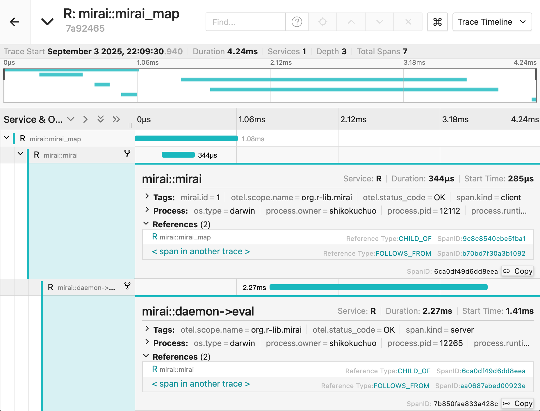
- See OpenTelemetry for details
- Works seamlessly with any OpenTelemetry-compatible observability platform, including:
- Grafana
- Pydantic Logfire
- Jaeger
- Any of those listed at https://otelsdk.r-lib.org/reference/collecting.html.
Example:
library(mirai) moo <- function() { s("*") |> elem_text() } scrape <- function(moo, x) { library(selenider) print(x) session <- selenider_session() open_url("https://r-project.org") moo() } daemons(2) mirai_map(c(1:10), scrape, .args = list(moo = moo))[] daemons(0)library(selenider)must be called inside ofscrapeforselenider_sessionto be found- I think you could have a
load_packagesfunction and aload_functionsfunction with the necessary packages and functions you need inside the main function. Then addload_packagesandload_functionsto .arg
- I think you could have a
moowill not be found unless it’s included in .args- x is the input for
c(1:10). The input for the vector doesn’t have to be the first argument. I think it just has to be one not included in .args
Example:
log_msg(sprintf("Starting parallel processing with %d workers", NUM_WORKERS))

# Start mirai daemons
daemons(NUM_WORKERS, dispatcher = TRUE)

results <- mirai_map(
  select(store_months, store_key, year, month),
  \(store_key, year, month) {
    library(dplyr)
    library(lubridate)
    library(quarto)

    generate_report(
      store_key = store_key,
      year = year,
      month = month
    )
  },
  generate_report = generate_report,
  OUTPUT_DIR = OUTPUT_DIR
)[.progress]

# Stop mirai daemons
daemons(0)

log_msg("Parallel processing complete")
- {purrr}
Uses {mirai} for parallelization, so
daemonsandin_parallelneededlibrary(purrr) library(mirai) # Set up 4 parallel processes daemons(4) # Define a slow model fitting function slow_lm <- function(formula, data) { Sys.sleep(0.1) # Simulate computational complexity lm(formula, data) } # Fit models to different subsets of data in parallel models <- mtcars |> split(mtcars$cyl) |> map(in_parallel(\(df) slow_lm(mpg ~ wt + hp, data = df), slow_lm = slow_lm)) daemons(0)Using nested functions
fn <- function(x) helper_fn(x) * 2 helper_fn <- function(x) x + 1 1:5 |> map(in_parallel(\(x) fn(x), fn = fn, helper_fn = helper_fn))- Also see ebtools::add_spatial_lags for a similar but more complex example
Explict dependencies required
my_data <- c(1, 2, 3)
map(1:3, in_parallel(\(x) mean(my_data), my_data = my_data))

map(1:3, in_parallel(\(x) vctrs::vec_init(integer(), x)))

map(1:3, in_parallel(\(x) {
  library(vctrs)
  vec_init(integer(), x)
}))
Distributed Compute
# Set up remote daemons on a Slurm HPC cluster
daemons(
  n = 100,
  url = host_url(),
  remote = cluster_config(command = "sbatch")
)

# Your purrr code remains exactly the same!
results <- big_dataset |>
  split(big_dataset$group) |>
  map(in_parallel(\(df) complex_analysis(df), complex_analysis = complex_analysis))

daemons(0)
Nested Functions (source)
daemons(4, output = TRUE) # `output = TRUE` lets you see the daemon output myprint <- function() { cat("inside myprint\n") } slow_lm <- function(formula, data, print_func) { # add helper function as an argument Sys.sleep(0.1) # Simulate computational complexity print_func() lm(formula, data) } models <- mtcars |> split(mtcars$cyl) |> map(in_parallel( \(df) slow_lm(mpg ~ wt + hp, data = df, myprint), # pass `myprint` as the helper function slow_lm = slow_lm, myprint = myprint )) daemons(0)- The nested function is an argument in the outer function that’s passed to
map
- The nested function is an argument in the outer function that’s passed to
MLflow
Misc
- Website, Repo, Docs, R API, Python API
- Resources
Tracking
Misc
mlflow_log_batch(df)- A dataframe with columns key, value, step, timestamp- Key can be names of metrics, params
- Step is probably for loops
- Timestamp can be from
Sys.time()probably
mlflow.search_runs()- querying runsAvailable columns greatly exceed those available in the experiments GUI
Example: py
# Create DataFrame of all runs in *current* experiment
df = mlflow.search_runs(order_by=["start_time DESC"])

# Print a list of the columns available
# print(list(df.columns))

# Create DataFrame with subset of columns
runs_df = df[
    [
        "run_id",
        "experiment_id",
        "status",
        "start_time",
        "metrics.mse",
        "tags.mlflow.source.type",
        "tags.mlflow.user",
        "tags.estimator_name",
        "tags.mlflow.rootRunId",
    ]
].copy()
runs_df.head()

# add additional useful columns
runs_df["start_date"] = runs_df["start_time"].dt.date
runs_df["is_nested_parent"] = runs_df[["run_id","tags.mlflow.rootRunId"]].apply(lambda x: 1 if x["run_id"] == x["tags.mlflow.rootRunId"] else 0, axis=1)
runs_df["is_nested_child"] = runs_df[["run_id","tags.mlflow.rootRunId"]].apply(lambda x: 1 if x["tags.mlflow.rootRunId"] is not None and x["run_id"] != x["tags.mlflow.rootRunId"]else 0, axis=1)
runs_df
- Use
mlflow.pyfuncfor a model agnostic Class approachAn approach which allows you to use libraries outside of {{sklearn}}
Example: Basic (source)
# Step 1: Create a mlflow.pyfunc model class ToyModel(mlflow.pyfunc.PythonModel): """ ToyModel is a simple example implementation of an MLflow Python model. """ def predict(self, context, model_input): """ A basic predict function that takes a model_input list and returns a new list where each element is increased by one. Parameters: - context (Any): An optional context parameter provided by MLflow. - model_input (list of int or float): A list of numerical values that the model will use for prediction. Returns: - list of int or float: A list with each element in model_input is increased by one. """ return [x + 1 for x in model_input] # Step 2: log this model as an mlflow run with mlflow.start_run(): mlflow.pyfunc.log_model( artifact_path = "model", python_model=ToyModel() ) run_id = mlflow.active_run # Step 3: load the logged model to perform inference model = mlflow.pyfunc.load_model(f"runs:/{run_id}/model") # dummy new data x_new = [1,2,3] # model inference for the new data print(model.predict(x_new)) >>> [2, 3, 4]- This only shows a predict method, but you can include anything you need such as a fit and preprocessing methods.
- See source for a more involved XGBoost model example and details on extracting metadata.
Set experiment name and get experiment id
- Syntax:
mlflow_set_experiment("experiment_name")- This might require a path e.g. “/experiment-name” instead the name
- Experiment IDs can be passed to
start_run()(see below) to ensure that the run is logged into the correct experimentExample: py
my_experiment = mlflow.set_experiment("/mlflow_sdk_test")
experiment_id = my_experiment.experiment_id
with mlflow.start_run(experiment_id=experiment_id):
- Syntax:
Starting runs
Using a
mlflow_log_function automatically starts a run, but then you have tomlflow_end_runUsing
with(mlflow_start_run(){})stops the run automatically once the code inside thewith()function is completedmlflow_start_run( run_id = NULL, experiment_id = only when run id not specified, start_time = only when client specified, tags = NULL, client = NULL)Example
library(mlflow)
library(glmnet)

# can format the variable outside the log_param fun or inside
alpha <- mlflow_param(args)

# experiment contained inside start_run
with(mlflow_start_run( ) {

    alpha_fl <- mlflow_log_param("alpha" = alpha)
    lambda_fl <- mlflow_log_param("lambda" = mlflow_param(args))

    mod <- glmnet(args)

    # preds
    # error

    # see Models section below for details
    mod_crate <- carrier::crate(~glmnet::glmnet.predict(mod, train_x), mod)
    mlflow_log_model(mod_crate, "model_folder")

    mlflow_log_metric("MAE", error)

})
# this might go on the inside if you're looping the "with" FUN and want to log results of each loop
mlflow_end_run()

# not working, logs run, but doesn't log metrics
# run saved script
mlflow::mlflow_run(entry_point = "script.R")
# End any existing runs mlflow.end_run() with mlflow.start_run() as run: # Turn autolog on to save model artifacts, requirements, etc. mlflow.autolog(log_models=True) print(run.info.run_id) diabetes_X = diabetes.data diabetes_y = diabetes.target # Split data into test training sets, 3:1 ratio ( diabetes_X_train, diabetes_X_test, diabetes_y_train, diabetes_y_test, ) = train_test_split(diabetes_X, diabetes_y, test_size=0.25, random_state=42) alpha = 0.9 solver = "cholesky" regr = linear_model.Ridge(alpha=alpha, solver=solver) regr.fit(diabetes_X_train, diabetes_y_train) diabetes_y_pred = regr.predict(diabetes_X_test) # Log desired metrics mlflow.log_metric("mse", mean_squared_error(diabetes_y_test, diabetes_y_pred)) mlflow.log_metric( "rmse", sqrt(mean_squared_error(diabetes_y_test, diabetes_y_pred))Custom run names
Example: py
# End any existing runs
mlflow.end_run()


# Explicitly name runs
today = dt.today()

run_name = "Ridge Regression " + str(today)

with mlflow.start_run(run_name=run_name) as run:
Previously unlogged metrics can be retrieved retroactively with the run id
# py with mlflow.start_run(run_id="3fcf403e1566422493cd6e625693829d") as run: mlflow.log_metric("r2", r2_score(diabetes_y_test, diabetes_y_pred))- The run_id can either be extracted by
print(run.info.run_id)from the previous run, or by queryingmlflow.search_runs()(See Misc above).
- The run_id can either be extracted by
Nested Runs
Useful for evaluating and logging parameter combinations to determine the best model (i.e. grid search), they also serve as a great logical container for organizing your work. With the ability to group experiments, you can compartmentalize individual data science investigations and keep your experiments page organized and tidy.
Example: py; start a nested run
# End any existing runs mlflow.end_run() # Explicitly name runs run_name = "Ridge Regression Nested" with mlflow.start_run(run_name=run_name) as parent_run: print(parent_run.info.run_id) with mlflow.start_run(run_name="Child Run: alpha 0.1", nested=True): # Turn autolog on to save model artifacts, requirements, etc. mlflow.autolog(log_models=True) diabetes_X = diabetes.data diabetes_y = diabetes.target # Split data into test training sets, 3:1 ratio ( diabetes_X_train, diabetes_X_test, diabetes_y_train, diabetes_y_test, ) = train_test_split(diabetes_X, diabetes_y, test_size=0.25, random_state=42) alpha = 0.1 solver = "cholesky" regr = linear_model.Ridge(alpha=alpha, solver=solver) regr.fit(diabetes_X_train, diabetes_y_train) diabetes_y_pred = regr.predict(diabetes_X_test) # Log desired metrics mlflow.log_metric("mse", mean_squared_error(diabetes_y_test, diabetes_y_pred)) mlflow.log_metric( "rmse", sqrt(mean_squared_error(diabetes_y_test, diabetes_y_pred)) ) mlflow.log_metric("r2", r2_score(diabetes_y_test, diabetes_y_pred))- alpha 0.1 is the parameter value being evaluated
Example: py; add child runs
# End any existing runs mlflow.end_run() with mlflow.start_run(run_id="61d34b13649c45699e7f05290935747c") as parent_run: print(parent_run.info.run_id) with mlflow.start_run(run_name="Child Run: alpha 0.2", nested=True): # Turn autolog on to save model artifacts, requirements, etc. mlflow.autolog(log_models=True) diabetes_X = diabetes.data diabetes_y = diabetes.target # Split data into test training sets, 3:1 ratio ( diabetes_X_train, diabetes_X_test, diabetes_y_train, diabetes_y_test, ) = train_test_split(diabetes_X, diabetes_y, test_size=0.25, random_state=42) alpha = 0.2 solver = "cholesky" regr = linear_model.Ridge(alpha=alpha, solver=solver) regr.fit(diabetes_X_train, diabetes_y_train) diabetes_y_pred = regr.predict(diabetes_X_test) # Log desired metrics mlflow.log_metric("mse", mean_squared_error(diabetes_y_test, diabetes_y_pred)) mlflow.log_metric( "rmse", sqrt(mean_squared_error(diabetes_y_test, diabetes_y_pred)) ) mlflow.log_metric("r2", r2_score(diabetes_y_test, diabetes_y_pred))- Add to nested run by using parent run id, e.g. run_id=“61d34b13649c45699e7f05290935747c”
- Obtained by
print(parent_run.info.run_id)from the previous run or querying viamlflow.search_runs(see below)
- Obtained by
- Add to nested run by using parent run id, e.g. run_id=“61d34b13649c45699e7f05290935747c”
Query Runs
Available columns greatly exceed those available in the experiments GUI
Example: py; Create Runs df
# Create DataFrame of all runs in *current* experiment
df = mlflow.search_runs(order_by=["start_time DESC"])


# Print a list of the columns available
# print(list(df.columns))


# Create DataFrame with subset of columns
runs_df = df[
    [
        "run_id",
        "experiment_id",
        "status",
        "start_time",
        "metrics.mse",
        "tags.mlflow.source.type",
        "tags.mlflow.user",
        "tags.estimator_name",
        "tags.mlflow.rootRunId",
    ]
].copy()
runs_df.head()


# add additional useful columns
runs_df["start_date"] = runs_df["start_time"].dt.date
runs_df["is_nested_parent"] = runs_df[["run_id","tags.mlflow.rootRunId"]].apply(lambda x: 1 if x["run_id"] == x["tags.mlflow.rootRunId"] else 0, axis=1)
runs_df["is_nested_child"] = runs_df[["run_id","tags.mlflow.rootRunId"]].apply(lambda x: 1 if x["tags.mlflow.rootRunId"] is not None and x["run_id"] != x["tags.mlflow.rootRunId"]else 0, axis=1)
runs_df
Query Runs Object
Example: Number of runs per start date
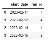
pd.DataFrame(runs_df.groupby("start_date")["run_id"].count()).reset_index()Example: How many runs have been tested for each algorithm?
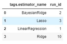
pd.DataFrame(runs_df.groupby("tags.estimator_name")["run_id"].count()).reset_index()
Projects
Name of the file is standard - “MLproject”
- yaml file but he didn’t give it an extension
- Multi-Analysis flows take the output of one script and input to another. The first script outputs the object somewhere in the working dir or a sub dir. The second script takes that object as a parameter with value = path.,
- e.g. dat.csv: path. See example https://github.com/mlflow/mlflow/tree/master/examples/multistep_workflow
Example
name: MyProject

envir: specify dependencies using packrat snapshot (didn't go into details)

entry points:
    # "main" is the default name used. Any script name can be an entry point name.
    main:
        parameters:
            # 2 methods, looks like same args as mlflow_param or mlflow_log_param
            # python types used, e.g. float instead of numeric used
            alpha: {type: float, default: 0.5}
            lambda:
                type: float
                default: 0.5
        # CLI commands to execute the script
        # sigh, he used -P in the video and -r on the github file
                # he used a -P for each param when executing from CLI, so that might be correct
                # Although that call to Rscript makes me think it might not be correct
        command: "Rscript <script_name>.R -P alpha={alpha} -P lambda={lambda}"
        # another one of their python examples
        command: "python etl_data.py --ratings-csv {ratings_csv} --max-row-limit {max_row_limit}"
        # This is similar to one of python their examples and it jives with Rscript practice, except there's a special function in the R script to take the args
        # command: "Rscript <script_name>.R {alpha} {lambda}"

    # second script, same format as 1st script
    validate:
        blah, blah
Run script with variable values from the CLI
mlflow mlflow run . --entry-point script.R -P alpha=0.5 -P lambda=0.7mlflowstarts mlflow.exe- . says run from current directory
- also guessing entry point value is a path from the working directory
Run script from github repo
$mlflow run https://github.com/ercbk/repo --entry-point script.R -P alpha=0.5 -P lambda=0.7- Adds link to repo in source col in ui for that run
- Adds link to commit (repo version) at the time of the run in the version col in the ui for that run
Models
Typically, models in R exist in memory and can be saved as .rds files. However, some models store information in locations that cannot be saved using save() or saveRDS() directly. Serialization packages can provide an interface to capture this information, situate it within a portable object, and restore it for use in new settings.
mlflow_save_modelcreates a directory with the bin file and a MLProject fileExamples
Using a function
mlflow_save_model(carrier::crate(function(x) { library(glmnet) # glmnet requires a matrix predict(model, as.matrix(x)) }, model = mod), "dir_name")predictusually takes a df but glmnet requires a matrix- model = mod is the parameter being passed into the function environment
- [dir_name][var.text] is the name of the folder that will be created
Using a lambda function
mlflow_save_model(carrier::crate(~glmnet::predict.glmnet(model, as.matrix(.x)), model = mod), "penal_glm")- Removed the library function (could’ve done that before as well)
- *** lambda functions require .x instead of just x ***
- The folder name is penal_glm
Serving a model as an API from the CLI
>> mlflow models serve -m file:penal_glmmlflowruns mlflow.exe- serve says create an API
- -m is for specifying the URI of the bin file
- Could be an S3 bucket
- file: says it’s a local path
- Default host:port 127.0.0.1:5000
- -h, -p can specify others
- *** Newdata needs to be in json column major format ***
Prediction is outputted in json as well
Example: Format in column major
jsonlite::toJSON(newdata_df, matrix = "columnmajor")Example: Send json newdata to the API
# CLI example for
curl http://127.0.0.1:5000/invocations -H 'Content-Type: application/json' -d '{    "columns": ["a", "b", "c"],    "data": [[1, 2, 3], [4, 5, 6]]}'
UI
mlflow_ui( )- Click date,
- metric vs runs
- notes
- artifact
- If running through github
- link to repo in source column for that run
- link to commit (repo version) at the time of the run in the version column
Targets
Misc
Also see
- Projects, Analyses >> Misc >> Analysis Workflow using {targets}
Tools
- tarborist - VScode/Positron extension. Static analysis for navigating and debugging complex R targets pipelines
- Hover over a target, and it tells you how many targets depend on it.
- Click on that number, and it lists them all.
- tarborist - VScode/Positron extension. Static analysis for navigating and debugging complex R targets pipelines
Notes from
Resources
- Docs, User Manual (ebook), Getting Started with targets in 4 min (Video)
- Working Smarter With targets (ebook)
- Carpentries Incubator: Targets Workshop
- Building Reproducible Analytical Pipelines in R, Ch.13
- Other chapters also mention targets
Modularizing Large Pipelines
- Using
sourceto load scripts where each may have multiple targets all associated with a particular component or step of the pipeline (e.g. loading mulitple datasets, fitting mulitple models, etc. (See discussion)
- Using
Set-Up
use_targets- Creates a “_targets.R” file in the project’s root directory
- Configures and defines the pipeline
- load packages
- HPC settings
- Load Functions from scripts
- Target pipeline
- Configures and defines the pipeline
- File has commented lines to guide you through the process
- Creates a “_targets.R” file in the project’s root directory
Project Structure Example
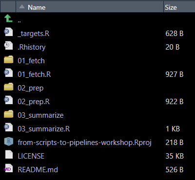
- Note the naming convention. Numbers indicate a step or phase in the pipeline
Target Pipeline
Basic Types
Target type Declaration Examples Object tar_targets(NAME,FUNCTION)Anything that can be an R object (e.g., plots, models, data.frames) File tar_targets(NAME,FUNCTION, format=”file”)Files (e.g., csv or png output files) Dynamic tar_targets(NAME,FUNCTION,pattern=map(VALUES))A series of object or file targets (e.g., a series of plots), one for each of the VALUESExample
# This file must be named _targets.R library(targets) source('R/myfunctions.R') tar_option_set(packages = c('biglm','tidyverse')) list( tar_target(file, "data.csv", format = "file"), tar_target(data, get_data(file)), tar_target(model, fit_model(data)), tar_target(plot, plot_model(model, data)) )- 1st arg is the target name (e.g. file, data, model, plot)
- 2nd arg is a function
- Function inputs are target names
- Except first target which has a file name for the 2nd arg
- “format” arg says that this target is a file and if the contents change, a re-hash should be triggered.
Loading multiple packages and functions (source)
suppressPackageStartupMessages(source("packages.R"))
for (f in list.files(here::here("R"), full.names = TRUE)) source (f)
Get a target from another project
withr::with_dir( "~/workflows/project_name/", targets::tar_load(project_name) )tar_make()- Finds_targets.Rand executes the pipeline- Output saved in _targets >> objects
Run
tar_makein the background- Put into .Rprofile in project
make <- function() {
    job::job(
        {{ targets::tar_make() }},
        title = "<whatever>"
    )
}
Operations
Check Pipeline
tar_manifest(fields = command)- lists names of targets and the functions to execute them
tar_visnetwork(targets_only = TRUE)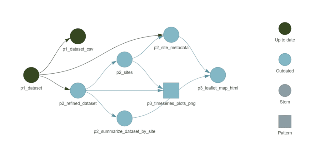
- Shows target dependency graph
- Could be slow if you have a lot of targets, so may want to comment in/out sections of targets and view them in batches.
- Target names reflect their phase (e.g.
p1_datasetindicates it belongs to Phase 1: fetching data). - File target names include a suffix for clarity (e.g.
p3_leaflet_map_htmlmakes it clear this target is an HTML file).
tar_read(target_name)- Reads the output of a target- e.g. If it’s a plot output, a plot will be rendered in the viewer.
Dask
Misc
Notes from Saturn Dask in the Cloud video
XGBoost, RAPIDS, LightGLM libraries can natively recognize Dask DataFrames and use parallelize using Dask
{{dask-ml}} can be used to simplify training multiple models in parallel
PyTorch DDP (Distributed Data Parallel)
- {{dask_pytorch_ddp}} for Saturn
- Each GPU has it’s own version of the model and trains concurrently on a data batch
- Results are shared between GPUs and a combined gradient is computed
from dask_pytorch_ddp import dispatch
futures = dispatch.run(dask_client, model_training_function)
Basic Usage
Dask Collections
- Dask DataFrames - Mimics Pandas DataFrames
- They’re essentially collection of pandas dfs spread across workers
- Dask Arrays - Mimics NumPy
- Dask Bags - Mimics map, filter, and other actions on collections
- Dask DataFrames - Mimics Pandas DataFrames
Storage
- Cloud storage (e.g. S3, EFS) can be queried by Dask workers
- Saturn also provides shared folders that attach directly to Dask workers.
Use Locally
import dask.dataframe as dd ddf = dd.read.csv("data/example.csv") ddf.groupby('col_name').mean().compute()computestarts the computation and collects the results.- Evidently other functions can have this effect (see example). Need to check docs.
- For a Local Cluster, the cluster = LocalCluster() and Client(cluster) commands are used. Recommende to initialize such a cluster only once in code using the Singleton pattern. You can see how it can be implemented in Python here. Otherwise, you will initialize a new cluster every launch;
Specify chunks and object type
from dask import dataframe as dd
ddf = dd.read_csv(r"FILEPATH", dtype={'SimillarHTTP': 'object'},blocksize='64MB')
Fit sklearn models in parallel
import joblib from dask.distributed import Client client = Client(processes=False) with joblib.parallel_backend("dask"): rf.fit(X_train, y_train)- Not sure if client is needed here
Evaluation Options
Dask Delayed
- For user-defined functions — allows dask to parallelize and lazily compute them
@dask.delayed
def double(x):
    return x*2

@dask.delayed
def add(x, y):
    return x + y

a = double(3)
b = double(2)
total = add(a,b) # chained delayed functions
total.compute() # evaluates the functions
Futures
Evaluated immediately in the background
Single function
def double(x):
    return x*2
future = client.submit(double, 3)
Iterable
learning_rates = np.arange(0.0005, 0.0035, 0.0005) futures = client.map(train_model, learning_rates) # map(function, iterable) gathered_futures = client.gather(futures) futures_computed = client.compute(futures_gathered, resources = {"gpu":1})- resources tells dask to only send one task per gpu-worker in this case
Monitoring
Logging
from distributed.worker import logger @dask.delayed def log(): logger.info(f'This is sent to the worker log') # ANN example logger.info( f'{datetime.datetime.now().isoformat(){style='color: #990000'}[}]{style='color: #990000'} - lr {lr} - epoch {epoch} - phase {phase} - loss {epoch_loss}' )- Don’t need a separate log function. You can just include
logger.infoin the model training function.
- Don’t need a separate log function. You can just include
Built-in dashboard
.png)
- Task Stream - each bar is a worker; colors show activity category (e.g. busy, finished, error, etc.)
Error Handling
The Dask scheduler will continue the computation and start another worker if one fails.
- If your code is what causing the error then it won’t matter
Libraries
import traceback
from distributed.client import wait, FIRST_COMPLETED
Create a queue of futures
queue = client.compute(results) futures_idx = {fut: i for i, fut in enumerate(queue)} results = [None for x in range(len(queue))]- Since we’re not passsing [sync = True]{arg-text}, we immediately get back futures which represent the computation that hasn’t been completed yet.
- Enumerate each item in the future
- Populate the “results” list with Nones for now
Wait for results
while queue:
    result = wait(queue, return_when = FIRST_COMPLETED)
Futures either succeed (“finished”) or they error (chunk included in while loop)
for future in result.done: index = futures_idx[future] if future.status == 'finished': print(f'finished computation #[{index}]{style='color: #990000'}') results[index] = future.result() else: print(f'errored #[{index}]{style='color: #990000'}') try: future.result() except Exception as e: results[index] = e traceback.print_exc() queue = result.not_done- future.status contains results of computation so you know what to retry
- Succeeds: Print that it finished and store the result
- Error: Store exception and print the stack trace
- Set queue to those futures that haven’t been completed
Optimization
- Resources
- Dask Dataframes Best Practices
- In general, recommends partition size of 100MB, but this doesn’t take into account server specs, dataset size, or application (e.g model fitting). Could be a useful starting point though.
- Dask Dataframes Best Practices
- Notes from:
- Almost Everything You Want to Know About Partition Size of Dask Dataframes
- Use Case: 2-10M rows using 8 to 16GB of RAM
- Almost Everything You Want to Know About Partition Size of Dask Dataframes
- Partition Size
- Issues
- Too Large: Takes too much time and resources to process them in RAM
- Too Small: To process all of them Dask needs to load these tables into RAM too often. Therefore, more time is spent on synchronization and uploading/downloading than on the calculations themselves
- Example: Runtime, 500K rows, 4 columns, XGBoost
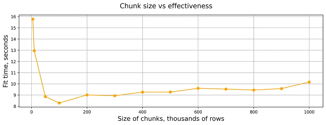
- Exact resource specs for this chart werent’ provided, but the experiment included 2, 3, and 4 vCPUs and 1, 2, and 4GB RAM per vCPU
- Issues
Cloud
Saturn
- Starting Dask from Jupyter Server that’s running JupyterLab, the Dask Cluster will have all the libraries loaded into Jupyter Server
- Options
- Saturn Cloud UI
- Once you start a Jupyter Server, there’s a button to click that allows you to specify and run a Dask Cluster
- Do work on a JupyterLab notebook
- Benefits
- In a shared environment
- Libraries automatically get loaded onto the Dask cluster
- Once you start a Jupyter Server, there’s a button to click that allows you to specify and run a Dask Cluster
- Programmatically (locally)
SSH into Jupyter Server (which is connected to the Dask Cluster) at Saturn
Connect directly to Dask Cluster at Saturn
Cons
- Have to load packages locally and on Jupyter Server and/or Dask Cluster
- Make sure versions/environments match
Connection (basic)
from dask_saturn import SaturnCluster
cluster = SaturnCluster()
client = Client(cluster)
- Saturn Cloud UI
- Example
From inside a jupyterlab notebook on a jupyter server with a dask cluster running
Imports
import dask.dataframe as dd
import numpy as np
from dask.diagnostics import ProgressBar
from dask.distributed import Client, wait
from dask_saturn import SaturnCluster
Start Cluster
n_workers = 3
cluster = SaturnCluster()
client = Client(cluster)
client.wait_for_workers(n_workers = n_workers) # if workers aren't ready, wait for them to spin up before proceding
client.restart()
For bigger tasks like training ANNs on GPUs, you to specify a gpu instance type (i.e. “worker_size”) and scheduler with plenty of memory
cluster = SaturnCluster( n_workers = n_workers, scheduler_size = 'large', worker_size = 'g3dnxlarge' )- If you’re bringing back sizable results from your workers, your scheduler needs plenty of RAM.
Upload Code files
1 file -
client.upload_file("functions.py")- Uploads a single file to all workers
Directory
from dask_saturn import RegesterFiles, sync_files client.register_worker_plugin(RegisterFiles()) sync_files(client, "functions") client.restart()- Plugin allows you to sync directory among workersjjj
Data
ddf = dd.read_parquet( "/path/to/file.pq" ) ddf = ddf.persist() _ = wait(ddf) # halts progress until persistance is done- Persist saves the data to the Dask workers
- Not necessary, but if you didn’t, then each time you call
.compute()you’d have to reload the file
- Not necessary, but if you didn’t, then each time you call
- Persist saves the data to the Dask workers
Do work
ddf["signal"] = ( ddf["ask_close"].rolling(5 * 60).mean() - ddf["ask_close"].rolling(20 * 60).mean() ) # ... blah, blah, blah ddf["total"] = ddf["return"].cumsum().apply(np.exp, meta = "return", "float64"))- Syntax just like pandas except:
- meta = (column, type) - Dask’s lazy computation sometimes gets column types wrong, so this specifies types explicitly
- Syntax just like pandas except:
Compute and bring back to client
total_returns = ddf["total"].tail(1) print(total_returns)- Evidently
.taildoes whatcomputeis supposed to do.
- Evidently
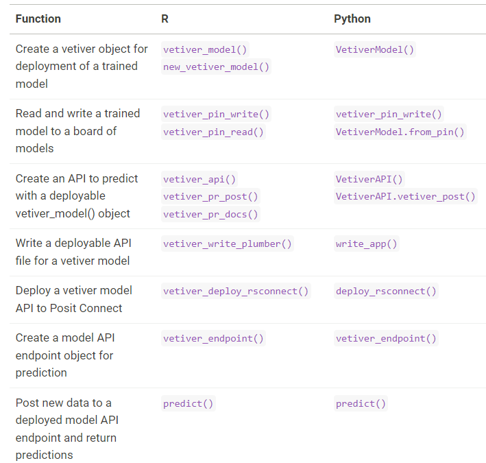
Vetiver
Misc
Helps with 3 aspects of MLOps
- Versioning
- Keeps track of metadata
- Helpful during retraining
- Deploying
- Utilizes REST APIs to serve models
- Monitoring
- Tracks model performance
- Versioning
Fit Workflow Object
model <-
  recipe(species ~ island + flipper_length_mm + body_mass_g,
    data = penguins_data) |>
  workflow(nearest_neighbor(mode = "classification")) |>
  fit(penguins_data)
Create a Vetiver Model Object
v_model <-
  vetiver::vetiver_model(model,
    model_name = "k-nn",
    description = "hyperparam-update-4")
v_model
#>
#> ── k-nn ─ <bundled_workflow> model for deployment
#> hyperparam-update-4 using 3 features
Versioning
Write model to a {pins} board (storage)
board <- pins::board_connect() board %>% vetiver_pin_write(v_model)board_*has many options including the major cloud providers- Here “connect” stands for Posit Connect
board_temp(versioned = TRUE)creates a temporary local folder and stores the serialized model there.
Create a REST API
library(plumber) pr() %>% vetiver_api(v_model) #> # Plumber router with 2 endpoints, 4 filters, and 1 sub-router. #> # Use `pr_run()` on this object to start the API. #> ├──[queryString] #> ├──[body] #> ├──[cookieParser] #> ├──[sharedSecret] #> ├──/logo #> │ │ # Plumber static router serving from directory: /Library/Frameworks/R.framework/Versions/4.2-arm64/Resources/library/vetiver #> ├──/ping (GET) #> └──/predict (POST) ## next pipe to `pr_run()` for local API- Then next step is pipe this into
pr_run()to start the API locally - Helpful for development or debugging
- Then next step is pipe this into
Test
Deploy locally
pr() %>% vetiver_api(v_model) |> pr_run()- When you run the code, a browser window will likely open. If it doesn’t simply navigate to
http://127.0.0.1:7764/__docs__/
- When you run the code, a browser window will likely open. If it doesn’t simply navigate to
Ping API
base_url <- "127.0.0.1:7764/"
url <- paste0(base_url, "ping")
r <- httr::GET(url)
metadata <- httr::content(r, as = "text", encoding = "UTF-8")
jsonlite::fromJSON(metadata)

#> $status
#> [1] "online"
#>
#> $time
#> [1] "2024-05-27 17:15:39"
Test
predictendpointurl <- paste0(base_url, "predict") endpoint <- vetiver::vetiver_endpoint(url) pred_data <- penguins_data |> dplyr::select("island", "flipper_length_mm", "body_mass_g") |> dplyr::slice_sample(n = 10) predict(endpoint, pred_data)- The API also has endpoints metadata and pin-url
Deploy
Using Docker
Create a docker file
vetiver::vetiver_prepare_docker( pins::board_connect(), "colin/k-nn", docker_args = list(port = 8080) )- Creates a docker file, renv.lock file, and plumber app that can be uploaded and deployed anywhere (e.g. AWS, GCP, digitalocean)
Build Image
docker build --tag my-first-model .Run Image
docker run --rm --publish 8080:8080 my-first-model
Without Docker
Posit Connect
vetiver::vetiver_deploy_rsconnect( board = pins::board_connect(), "colin/k-nn" )vetiver_deploy_sagemaker()also available
Monitor
Score model on new data and write metrics to storage
new_metrics <- augment(x = v, # model API endpoint object new_data = housing_val) %>% vetiver_compute_metrics(date_var = date, period = "week", truth = price, estimate = .pred) vetiver_pin_metrics( board, new_metrics, "julia.silge/housing-metrics", overwrite = TRUE ) #> # A tibble: 90 × 5 #> .index .n .metric .estimator .estimate #> <dttm> <int> <chr> <chr> <dbl> #> 1 2014-11-02 00:00:00 224 rmse standard 206850. #> 2 2014-11-02 00:00:00 224 rsq standard 0.413 #> 3 2014-11-02 00:00:00 224 mae standard 140870. #> 4 2014-11-06 00:00:00 373 rmse standard 221627. #> 5 2014-11-06 00:00:00 373 rsq standard 0.557 #> 6 2014-11-06 00:00:00 373 mae standard 150366. #> 7 2014-11-13 00:00:00 427 rmse standard 255504. #> 8 2014-11-13 00:00:00 427 rsq standard 0.555 #> 9 2014-11-13 00:00:00 427 mae standard 147035. #> 10 2014-11-20 00:00:00 376 rmse standard 248405. #> # ℹ 80 more rows- date_var: The name of the date column to use for monitoring the model performance over time.
- period: The period (“hour”, “day”, “week”, etc) over which the scoring metrics should be computed.
- truth: The actual values of the target variable
- estimate: The predictions of the target variable to compare the actual values against
Analyze metrics
new_metrics %>%
  ## you can operate on your metrics as needed:
  filter(.metric %in% c("rmse", "mae"), .n > 20) %>%
  vetiver_plot_metrics() +
  ## you can also operate on the ggplot:
  scale_size(range = c(2, 5))