Modeling
Misc
- {{flowcluster} - Functions for clustering origin-destination (OD) pairs, representing desire lines (or flows).
- Includes:
- Creating distance matrices between OD pairs
- Passing distance matrices to a clustering algorithm
- The current distance matrix is an implementation of the flow distance and flow dissimilarity measures
- Can aggregate the flows in each cluster into a single line representing the average flow direction and magnitude
- Includes:
- {geocmeans} - Apply Spatial Fuzzy c-means Algorithm, visualize and interpret results. This method is well suited when the user wants to analyze data with a fuzzy clustering algorithm and to account for the spatial dimension of the dataset.
- In addition, indexes for measuring the spatial consistency and classification quality are proposed
- {gsClusterDetect} - Utilities for Geospatial Cluster Detection and Significance Classification
- Provides utilities for manipulating time series of location-based counts of events to detect geospatial clusters.
- Significance of these clusters is determined using a set of models that classify based on a learned relationship between observed and the log(observed/expected) ratio of counts.
- {GWnnegPCA} - Geographically Weighted Non-Negative Principal Components Analysis
- {lagsarlmtree} - Model-based linear model trees adjusting for spatial correlation using a simultaneous autoregressive spatial lag
- The linear model is a SLM econometric spatial regression model imported from spatialreg (See Regression, Spatial >> Econometric)
- {loopevd} - Performs extreme value analysis at multiple locations using functions from the ‘evd’ package. Supports both point-based and gridded input data using the ‘terra’ package, enabling flexible looping across spatial datasets for batch processing of generalised extreme value, Gumbel fits
- {mlr3spatial} - Extends the ‘mlr3’ ML framework with methods for spatial objects. Data storage and prediction are supported for packages ‘terra’, ‘raster’ and ‘stars’.
- {RandomForestsGLS} - Generalizaed Least Squares RF
- Takes into account the correlation structure of the data. Has functions for spatial RFs and time series RFs
- {sfclust} - Bayesian Spatial Functional Clustering
- {SLGP} - Spatial Logistic Gaussian Process for Field Density Estimation
- Can be used for density prediction, quantile and moment estimation, sampling methods, and preprocessing routines for basis functions.
- Applications arise in spatial statistics, machine learning, and uncertainty quantification.
- {spatialAtomizeR} - Implements atom-based regression models (ABRM) for analyzing spatially misaligned data.
- i.e. response and some covariates are at one resolution or set of boundaries and the other covariates are at another resolution or set of boundaries. The area units are not nested. (e.g. not like counties and states)
- Provides functions for simulating misaligned spatial data, preparing NIMBLE model inputs, running MCMC diagnostics, and comparing different spatial analysis methods including dasymetric mapping.
- {SpatialDownscaling} - Methods for Spatial Downscaling Using Deep Learning
- The aim of the spatial downscaling is to increase the spatial resolution of the gridded geospatial input data.
- Contains two deep learning based spatial downscaling methods: super-resolution deep residual network (SRDRN) and UNet (Paper)
- Can optionally account for cyclical temporal patterns in case of spatio-temporal data
- {spatialfusion} - Multivariate Analysis of Spatial Data Using a Unifying Spatial Fusion Framework
- {spatialRF} - Explanatory spatial regression models by combining Random Forest with spatial predictors that help the model reduce the spatial autocorrelation of the residuals and return honest variable importance scores.
- {spNNGP} (Vignette) - Provides a suite of spatial regression models for Gaussian and non-Gaussian point-referenced outcomes that are spatially indexed. The package implements several Markov chain Monte Carlo (MCMC) and MCMC-free nearest neighbor Gaussian process (NNGP) models for inference about large spatial data.
- {spVarBayes} (Paper, Tutorial) - Provides scalable Bayesian inference for spatial data using Variational Bayes (VB) and Nearest Neighbor Gaussian Processes (NNGP). All methods are designed to work efficiently even with 100,000 spatial locations, offering a practical alternative to traditional MCMC.
- Models
- spVB-MFA, spVB-MFA-LR, and spVB-NNGP. All three use NNGP priors for the spatial random effects, but differ in the choice of the variational families.
- spVB-NNGP uses a correlated Gaussian variational family with a nearest neighbor-based sparse Cholesky factor of the precision matrix.
- spVB-MFA and spVB-MFA-LR use a mean-field approximation variational family.
- Additionally, spVB-MFA-LR applies a one-step linear response correction to spVB-MFA for improved estimation of posterior covariance matrix, mitigating the well-known variance underestimation issue of mean-field approximation
- Allows for covariates (i.e., fixed effects), enabling inference on the association of these with the outcome via the variational distribution of the regression coefficients. Variational distributions for the spatial variance and random error variance are also estimated, as in a fully Bayesian practice
- Simulation studies demonstrate that spVB-NNGP and spVB-MFA-LR outperform the existing variational inference methods in terms of both accuracy and computational efficiency. both spVB-NNGP and spVB-MFA-LR produce inference on the fixed and random effects that align closely with those obtained from the MCMC-based spNNGP, but at reduced computational cost.
- Models
- {tulpaMesh} - Generate constrained Delaunay triangulation meshes for use with stochastic partial differential equation (SPDE) spatial models
- {varycoef} - Implements a maximum likelihood estimation (MLE) method for estimation and prediction of Gaussian process-based spatially varying coefficient (SVC) models
- {vmsae} - Variational Autoencoded Multivariate Spatial Fay-Herriot model for efficiently estimating population parameters in small area estimation
Notes from
Resources
- Geocomputation with R, Ch.12
- Spatial Microsimulation with R - Teaches techniques for generating and analyzing spatial microdata to get the ‘best of both worlds’ from real individual and geographically-aggregated data
- Spatial Microdata Simulations are:
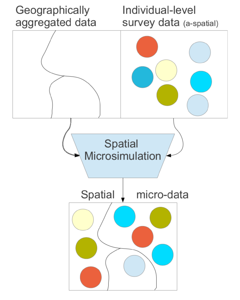
- Approximations of individual level data at high spatial resolution by combining individual and geographically aggregated datasets.: people allocated to places. (i.e. population synthesis)
- An approach to understanding multi level phenomena based on spatial microdata — simulated or real
- Geographically aggregated data are called constraints and the individual level survey data are called microdata
- Spatial Microdata Simulations are:
- Applied Machine Learning Using mlr3 in R, Ch.13.5
Papers
- A multivariate spatial model for ordinal survey-based data ({nimble} Code)
- Soil texture prediction with Bayesian generalized additive models for spatial compositional data
- Uses {brms} to fit a Bayesian GAM to model a compositional response. Model includes variables for elevation, slope, longitude, latitude
CV
- A common case is where sample data are collected opportunistically (“whatever could be found”), and are then used in a predictive framework that does not weight them.
- This has a consequence that the resulting model may be biased towards over-represented areas (in predictor space and/or in spatial coordinates space), and that simple (random) cross-validation statistics may be over-optimistic when taken as performance measures for spatial prediction
- Adaptive cross-validation measures such as spatial cross-validation may help getting more relevant measures for predictive performance.
- Standard CV methods
- For clustered data and interpolative and predictive use cases, it generally leads to overoptimistic performance metrics when the data has significant spatial autocorrelation.
- For random and regular distributed data and interpolative and predictive use cases, correctly ranked the models even when the data has significant spatial autocorrelation.
- Spatial CV Types: Spatial Blocking, Clustering, Sampling-Intensity-Weighted CV, Model-based Geostatistical Approaches, k-fold nearest neighbour distance matching (kNNDM) CV
- Spatial Resampling
Creates cross-validation folds by k-means clustering coordinate variables
library(tidymodels)
library(spatialsample)
set.seed(123)
spatial_splits <- spatial_clustering_cv(landslides, coords = c("x", "y"), v = 5)

# fit a logistic model
glm_spec <- logistic_reg()
lsl_form <- lslpts ~ slope + cplan + cprof + elev + log10_carea
lsl_wf <- workflow(lsl_form, glm_spec)
doParallel::registerDoParallel()
regular_rs <- fit_resamples(lsl_wf, bad_folds)
- A common case is where sample data are collected opportunistically (“whatever could be found”), and are then used in a predictive framework that does not weight them.
Design-based Approach: Assumes data comes from (spatially) random sampling (randomness in the sample locations), and we are interested in estimating means or totals
- Most standard machine learning methods, assume sample data to be independent which can be valid hen samples are collected by spatially random sampling over the spatial target area
- Uses when:
- Observations were collected using a spatial random sampling process
- Aggregated properties of the entire sample region (or sub-region) are needed
- Estimates are required that are not sensitive to model misspecification, for instance when needed for regulatory or legal purposes
Model-basd Approach: Assumes observations were not sampled randomly, or our interest is in predicting values at specific locations (mapping)
- When predictions for fixed locations are required, a model-based approach is needed and typically some form of spatial and/or temporal autocorrelation of residuals must be assumed.
- Use when:
- Predictions are required for individual locations, or for areas too small to be sampled
- The available data were not collected using a known random sampling scheme (i.e., the inclusion probabilities are unknown, or are zero over particular areas and or times)
Ways to Account for Spatial Autocorrelation
- Add spatial proxies as predictors
- Models
- Generalized-Least-Squares-style Random Gorest (RF–GLS) - Relaxes the independence assumption of the RF model
- Accounts for spatial dependencies in several ways:
- Using a global dependency-adjusted split criterion and node representatives instead of the classification and regression tree (CART) criterion used in standard RF models
- Employing contrast resampling rather than the bootstrap method used in a standard RF model
- Applying residual kriging with covariance modeled using a Gaussian process framework
- From the spatial proxies paper:
- “Outperformed or was on a par with the best-performing standard RF model with and without proxies for all parameter combinations in both the interpolation and extrapolation areas of the simulation study.”
- “The most relevant performance gains when comparing RF–GLS to RFs with and without proxies were observed in the ‘autocorrelated error’ scenario for the interpolation area with regular and random samples, where the RMSE was substantially lower.”
- Accounts for spatial dependencies in several ways:
- Generalized-Least-Squares-style Random Gorest (RF–GLS) - Relaxes the independence assumption of the RF model
Spatial Proxies
- Notes from Random forests with spatial proxies for environmental modelling: opportunities and pitfalls
- Spatial proxies are a set of spatially indexed variables with long or infinite autocorrelation ranges that are not causally related to the response.
- They are “proxy” since these predictors act as surrogates for unobserved factors that can cause residual autocorrelation, such as missing predictors or an autocorrelated error term.
- Types
- Geographical or Projected Coordinates
- Euclidean Distance Fields (EDFs)(i.e. distance-to variables?)
- Adding distance fields for each of the sampling locations (distance from one location to the other?), i.e. the number of added predictors equals the sample size.
- RFsp
- Tends to give worse results than coordinates when use of spatial proxies is inappropriate for either interpolation or extrapolation.
- But, together with EDFs, it is likely to yield the largest gains when the use of proxies is beneficial.
- Factors that could affect the effectiveness of spatial proxies
- Model Objectives
- Interpolation - There is a geographical overlap between the sampling and prediction areas
- The addition of spatial proxies to tree models such as RFs may be beneficial in terms of enhancing predictive accuracy, and they might outperform geostatistical or hybrid methods
- For Random or Regular spatial distributions of locations, the model should likely benefit, especially if there’s a large amount of spatial autocorrelation.
- For clustered spatial distributions of locations
- For weakly clustered data, strong spatial autocorrelation, and when there’s only a subset of informative predictors or no predictors at all, then models can expect some benefit.
- For other cases of weakly clustered data, there’s likely no affect or a little worse performance.
- For strongly clustered data , it probably worsens performance.
- For weakly clustered data, strong spatial autocorrelation, and when there’s only a subset of informative predictors or no predictors at all, then models can expect some benefit.
- Prediction (aka Extrapolation, Spatial-Model Transferability) - The model is applied to a new disjoint area
- The use of spatial proxies appears to worsen performance in all cases.
- Inference (aka Predictive Inference) - Knowledge discovery is the main focus
- Inclusion of spatial proxies has been discouraged
- Proxies typically rank highly in variable-importance statistics
- High-ranking proxies could hinder the correct interpretation of importance statistics for the rest of predictors, undermining the possibility of deriving hypotheses from the model and hampering residual analysis
- Interpolation - There is a geographical overlap between the sampling and prediction areas
- Large Residual Autocorrelation
- Better performance of models with spatial proxies is expected when residual dependencies are strong.
- Spatial Distribution
- Clustered samples frequently shown as potentially problematic for models with proxy predictors
- Including highly autocorrelated variables, such as coordinates with clustered samples, can result in spatial overfitting
- Model Objectives
Interaction Modeling
- Similar to interpolation but keeps the original spatial units as interpretive framework. Hence, the map reader can still rely on a known territorial division to develop its analyses
- They produce understandable maps by smoothing complex spatial patterns
- They enrich variables with contextual spatial information.
- Notes from {potential} documentation
- Packages
- There are two main ways of modeling spatial interactions: the first one focuses on links between places (flows), the second one focuses on places and their influence at a distance (potentials).
- Use Cases
- Retail Market Analysis: A national retail chain planning expansion in a metropolitan area would use potential models to identify optimal new store locations. The analysis would calculate the “retail potential” at various candidate sites
- Based on:
- Population density in surrounding neighborhoods
- Income levels (as a proxy for purchasing power)
- Distance decay function (people are less likely to travel farther to shop)
- Existing competitor locations
- Calculate distance matrix from potential site to competitor location
- Result:
- A retail chain might discover that a location with moderate nearby population but situated along major commuter routes has higher potential than a site with higher immediate population but poor accessibility. T
- The potential model would create a continuous surface showing retail opportunity across the entire region, with the highest values indicating prime locations for new stores
- Based on:
- Transportation Planning: Regional transportation authorities use potential models to optimize transit networks.
- They would:
- Map population centers (origins) and employment centers (destinations)
- Calculate interaction potential between all origin-destination pairs
- Weight these by population size and employment opportunities
- Apply distance decay functions reflecting willingness to commute
- Result:
- The resulting model might reveal corridors with high interaction potential but inadequate transit service. For instance, a growing suburban area might show strong potential interaction with a developing business district, but existing transit routes might follow outdated commuting patterns.
- The potential model helps planners identify where new bus routes, increased service frequency, or even rail lines would best serve actual travel demand.
- They would:
- Hospital Accessibility Study: Public health departments use potential models to identify healthcare deserts.
- They would:
- Map existing hospital and clinic locations with their capacity (beds, specialties)
- Calculate accessibility potential across the region
- Weight by demographic factors (elderly population, income levels)
- Apply appropriate distance decay functions (emergency vs. specialist care have different distance tolerances)
- Result:
- The model might reveal that while a rural county appears to have adequate healthcare on paper (population-to-provider ratio), the spatial distribution creates areas with extremely low healthcare potential.
- This analysis could justify mobile clinics, telemedicine investments, or targeted subsidies for new healthcare facilities in specific locations to maximize population benefi
- They would:
- Retail Market Analysis: A national retail chain planning expansion in a metropolitan area would use potential models to identify optimal new store locations. The analysis would calculate the “retail potential” at various candidate sites
- Comparisons ({potential}article)
- GDP per capita (cloropleth)
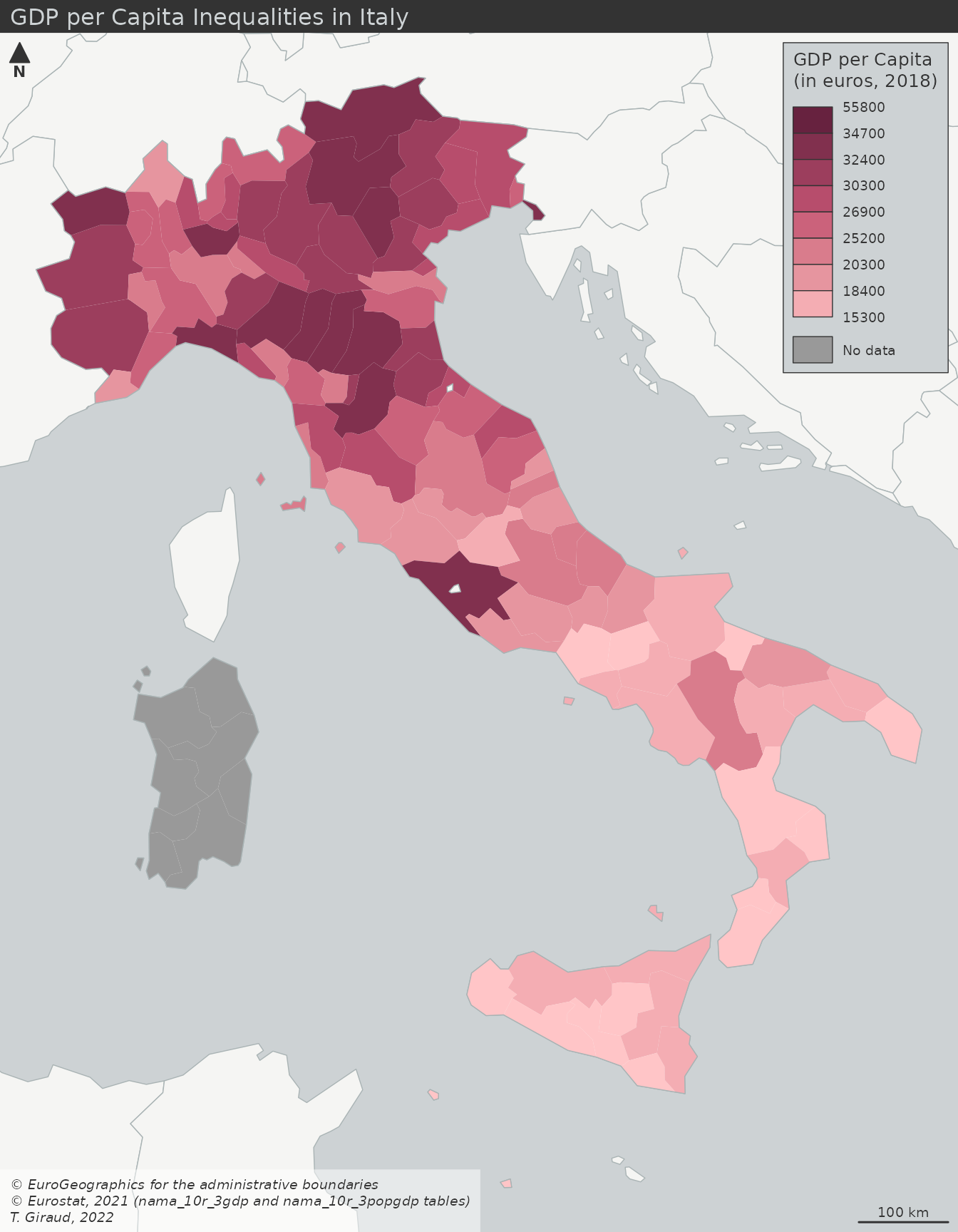
- Typical cloropleth at the municipality level
- Values have been binned
- Potential GDP per Capita (interaction)
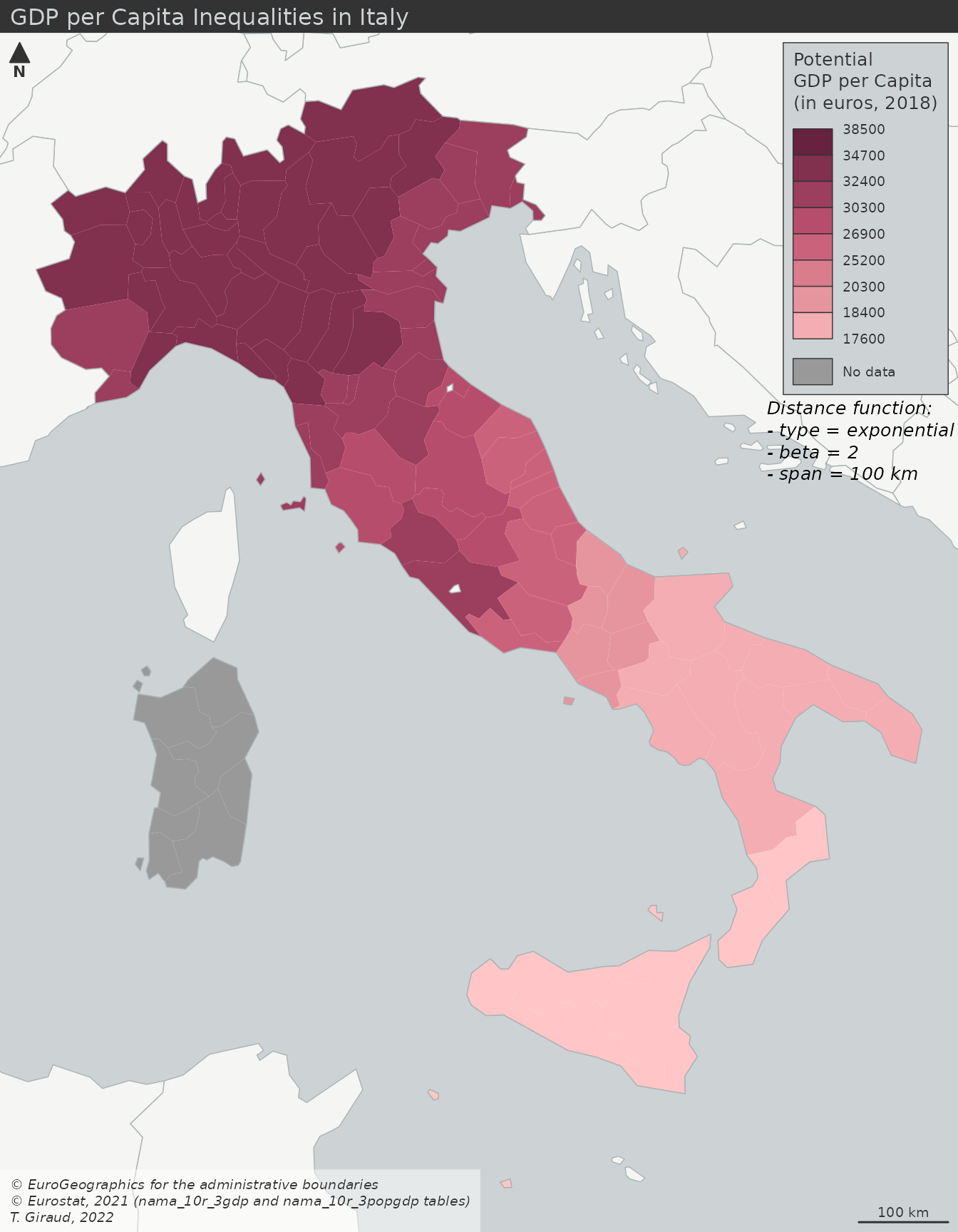
- Stewart Potentials have smoothed the values
- Municipality boundaries still intact, so you could perform an analysis based on these GDP regions
- Smoothed GDP per Capita (interpolation)
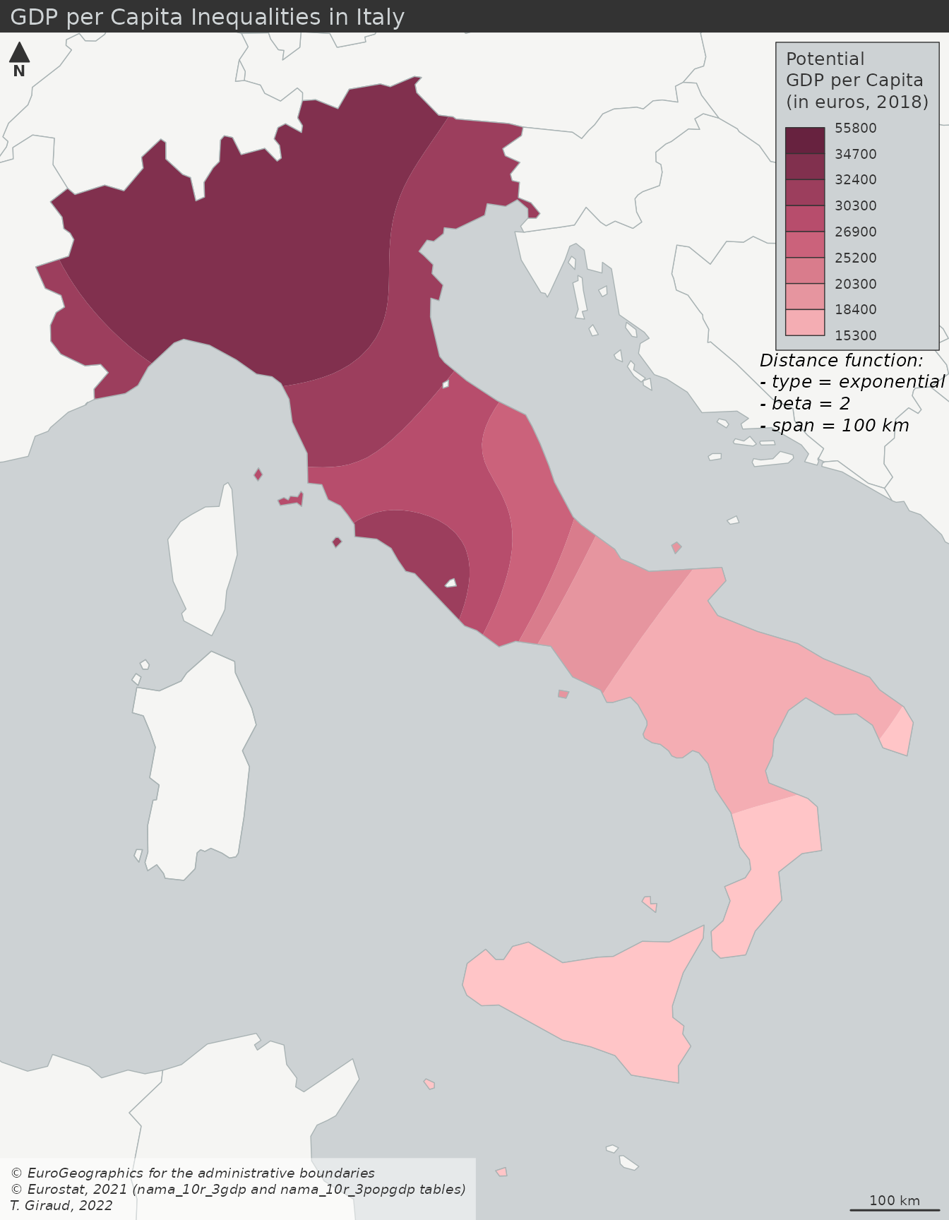
- Similar results as the interaction model except there are no boundaries
- GDP per capita (cloropleth)
Interpolation
Misc
The process of using points with known values to estimate values at other points. In GIS applications, spatial interpolation is typically applied to a raster with estimates made for all cells. Spatial interpolation is therefore a means of creating surface data from sample points.
Packages
- {BMEmapping} - Spatial Interpolation using Bayesian Maximum Entropy (BME)
- Ssupports optimal estimation using both precise (hard) and uncertain (soft) data, such as intervals or probability distributions
- {gstat} - OG; Has idw and various kriging methods.
- {intamap} (Paper) - Procedures for Automated Interpolation (Edzer Pebesma et al)
- One needs to choose a model of spatial variability before one can interpolate, and experts disagree on which models are most useful.
- {interpolateR} - Includes a range of methods, from traditional techniques to advanced machine learning approaches
- Inverse Distance Weighting (IDW): A widely used method that assigns weights to observations based on their inverse distance.
- Cressman Objective Analysis Method (Cressman): A powerful approach that iteratively refines interpolated values based on surrounding observations.
- RFmerge: A Random Forest-based method designed to merge multiple precipitation products and ground observations to enhance interpolation accuracy.
- RFplus: A novel approach that combines Random Forest with Quantile Mapping to refine interpolated estimates and minimize bias.
- {mbg} - Interface to run spatial machine learning models and geostatistical models that estimate a continuous (raster) surface from point-referenced outcomes and, optionally, a set of raster covariates
- {spatialize} (Paper) - Implements ensemble spatial interpolation, a novel method that combines the simplicity of basic interpolation methods with the power of classical geoestatistical tools
- Stochastic modelling and ensemble learning, making it robust, scalable and suitable for large datasets.
- Provides a powerful framework for uncertainty quantification, offering both point estimates and empirical posterior distributions.
- It is implemented in Python 3.x, with a C++ core for improved performance.
- {BMEmapping} - Spatial Interpolation using Bayesian Maximum Entropy (BME)
Resources
In Spatial Filtering or Smoothing, the unobserved values (\(S(s)\)) are simulated and a white noise component (\(\epsilon\)) (possibly reflecting measuerment error) is included such that
\[Z(s) = S(s) + \epsilon\]
- In Kriging, \(Z(s)\) is estimated through a model
Measurements can have strong regional variance, so the geographical distribution of measurements can have a strong influence on statistical estimates.
- Example: Temperature
- Two different geographical distributions of sensors

- A concentration of sensors in North can lead to a cooler average regional temperature and vice versa for the South.
- Distribution of temperatures across the region for 1 day.
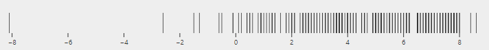
- With this much variance in temperature, a density of sensors in one area can distort the overall average.
- Interpolation evens out the geographical distribution of measurments
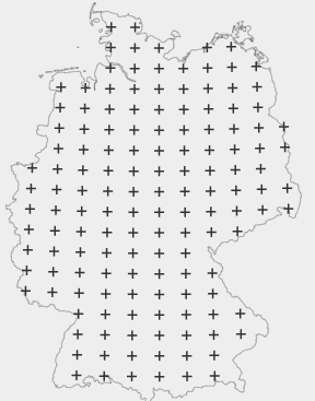
- Two different geographical distributions of sensors
- Example: Temperature
Inverse Distance Weighted (IDW)
IDW (inverse distance weighted) and Spline interpolation tools are referred to as deterministic interpolation methods because they are directly based on the surrounding measured values or on specified mathematical formulas that determine the smoothness of the resulting surface
A weighted average, using weights inverse proportional to distances from the interpolation location
\[\begin{align} &\hat z(s_0) = \frac{\sum_{i=1}^m w_i z(s_i)}{\sum_{i=1}^n w_i} \\ &\text{where} \;\; w_i = |s_o - s_i|^{-p} \end{align}\]
- \(p\) : The inverse distance power which is typically 2 or optimized via CV
Example: NO2 in Germany
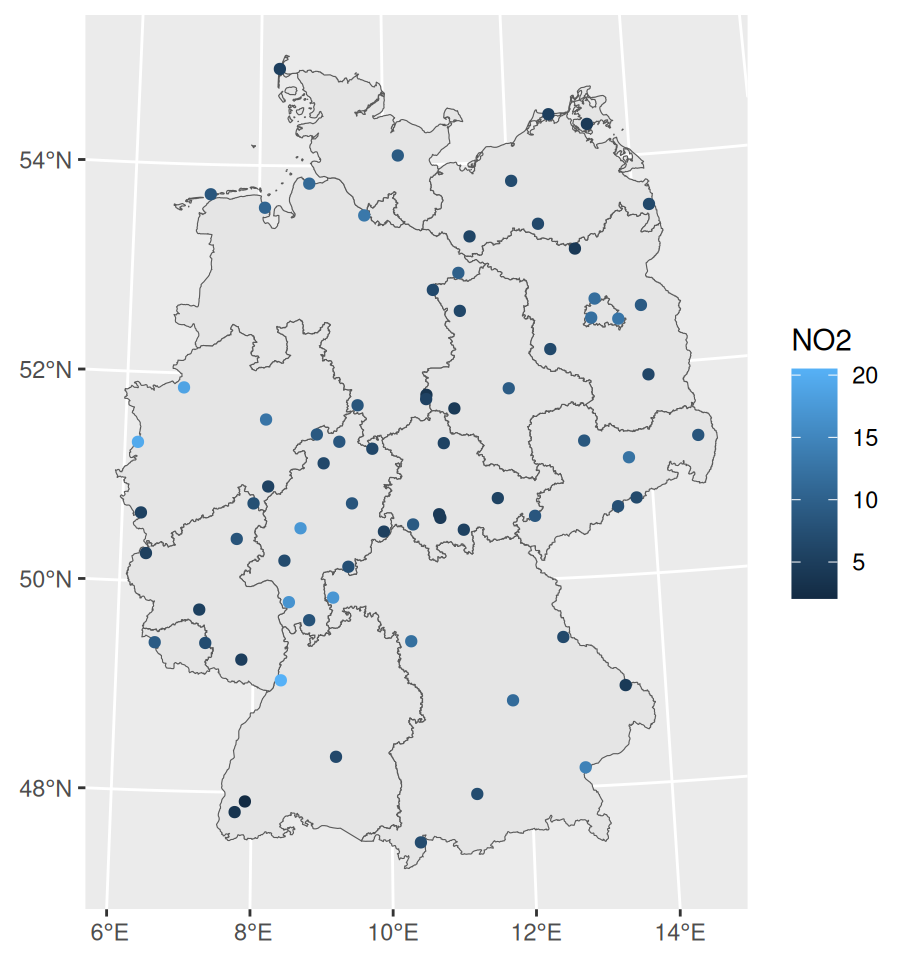
pacman::p_load( ggplot2, sf, stars, gstat ) dat_no2 <- readr::read_csv(system.file("external/no2.csv", package = "gstat"), show_col_types = FALSE) crs <- st_crs("EPSG:32632") shp_de <- read_sf("https://raw.githubusercontent.com/edzer/sdsr/main/data/de_nuts1.gpkg") |> st_transform(crs) sf_no2 <- st_as_sf(dat_no2, crs = "OGC:CRS84", coords = c("station_longitude_deg", "station_latitude_deg")) |> st_transform(crs) ggplot() + # germany shapefile geom_sf(data = shp_de) + # locations colored by value geom_sf(data = sf_no2, aes(color = NO2))- The variable of interest is values of NO2 pollution at various locations in Germany
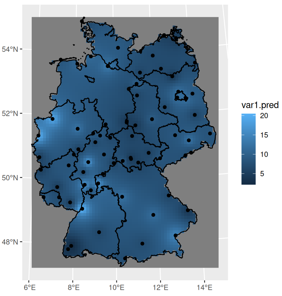
grid_de <- st_bbox(shp_de) |> st_as_stars(dx = 10000) |> st_crop(shp_de) idw_no2 <- idw(NO2 ~ 1, sf_no2, grid_de) ggplot() + # interpolation fill geom_stars( data = idw_no2, aes(x = x, y = y, fill = var1.pred) ) + # shapefile as a string geom_sf(data = st_cast(shp_de, "MULTILINESTRING")) + # locations geom_sf(data = sf_no2) + xlab(NULL) + ylab(NULL)- IDW requires a grid. dx says the cells of the grid have 10000m (10km) width which results in 10km x 10km cells.
- The grid isn’t very fine and is visible if you zoom-in.
- NO2 ~ 1 specifies an intercept-only (unknown, constant mean) model for (aka ordiary kriging model)
- The polygons as strings looks janky (esp zoomed in), but this code this way doesn’t work otherwise. I’m sure there has to be a way to do this with polygons though.
- The ordering of the layers is important. The interpolation fill must be first.