GLM

Misc

The degrees of freedom are related to the number of observations, and how many predictors you have used. If you look at the mean value in the prostate dataset for recurrence, it is 0.1708861, which means that 17% of the participants experienced a recurrence of prostate cancer. If you are calculating the mean of 315 of the 316 observations, and you know the overall mean of all 315, you (mathematically) know the value of the last observation - recurrence or not - it has no degrees of freedom. So for 316 observations, you have n-1 or 315, degrees of freedom. For each predictor in your model you ‘use up’ one degree of freedom. The degrees of freedom affect the significance of the test statistic (T, or chi-squared, or F statistic).
- Should be in the summary of the model
Chi Square test for the deviance only works for nested models
** The formulas for the deviances for a logistic regression model are slightly different since the deviance for the saturated logistic regression model is 0 **

Separation

Complete or quasi-complete separation occurs when there is a combination of regressors in the model whose value can perfectly predict one or both outcomes. In such cases, and such cases only, the maximum likelihood estimates and the corresponding standard errors are infinite.
Causes infinite estimates in binary regression models and for other models with a point mass at the bounday (typically at zero) such as Poisson and Tobit.
Bias-reduction methods used in {brglm2} or {brtobit} can be a remedy

Example: Logistic Regression (source)

Model

library("brglm2")
data("endometrial", package = "brglm2")
modML <- 
  glm(HG ~ NV + PI + EH, 
      family = binomial("logit"), 
      data = endometrial)
summary(modML)
#> 
#> Call:
#> glm(formula = HG ~ NV + PI + EH, family = binomial("logit"), 
#>     data = endometrial)
#> 
#> Deviance Residuals: 
#>      Min        1Q    Median        3Q       Max  
#> -1.50137  -0.64108  -0.29432   0.00016   2.72777  
#> 
#> Coefficients:
#>               Estimate Std. Error z value Pr(>|z|)    
#> (Intercept)    4.30452    1.63730   2.629 0.008563 ** 
#> NV            18.18556 1715.75089   0.011 0.991543    
#> PI            -0.04218    0.04433  -0.952 0.341333    
#> EH            -2.90261    0.84555  -3.433 0.000597 ***
#> ---
#> Signif. codes:  0 '***' 0.001 '**' 0.01 '*' 0.05 '.' 0.1 ' ' 1
#> 
#> (Dispersion parameter for binomial family taken to be 1)
#> 
#>     Null deviance: 104.903  on 78  degrees of freedom
#> Residual deviance:  55.393  on 75  degrees of freedom
#> AIC: 63.393
#> 
#> Number of Fisher Scoring iterations: 17

The standard error for NV is extremely large which makes it likely that separation has occurred

Verify Separation

# install.packages("detectseparation")
library("detectseparation")
update(modML, method = "detect_separation")
#> Implementation: ROI | Solver: lpsolve 
#> Separation: TRUE 
#> Existence of maximum likelihood estimates
#> (Intercept)          NV          PI          EH 
#>           0         Inf           0           0 
#> 0: finite value, Inf: infinity, -Inf: -infinity

Separation: TRUE and NV’s parameter is infinite (INF) confirms separation

Deviance Metrics

Misc
- Notes from Saturated Models and Deviance video
- Deviance is 2 * Log Likelihood
  - Log likelihood can usually be extracted from the model object (e.g. ll_proposed <- mod$logLik)
- Saturated Model also called the Full model (Also see Regression, Discrete >> Misc)
  - The full model has a parameter for each observation and describes the data perfectly while the reduced model provides a more concise description of the data with fewer parameters.
  - Usually calculated from the data themselves
```
data(wine, package = "ordinal")
tab <- with(wine, table(temp:contact, rating))
## Get full log-likelihood (aka saturated model log-likelihood)
pi.hat <- tab / rowSums(tab)
(ll.full <- sum(tab * ifelse(pi.hat > 0, log(pi.hat), 0))) ## -84.01558
```
- GOF: as a rule of thumb, if the deviance about the same size as the difference in the number of parameters (i.e. pfull - pproposed), there is NOT evidence of lack of fit. ({ordinal} vignette, pg 14)
  - Example (have doubts this is correct)
    - Looking at the number of params (“no.par”) for fm1 in Example: {ordinal}, model selection with LR tests below and the model summary in Proportional Odds (PO) >> Example: {ordinal}, response = wine rating (1 to 5 = most bitter), the number of parameters for the reduced model is the number of regression parameters (2) + number of thresholds (4)
    - For the full model (aka saturated), the number of thresholds should be the same, and there should be one more regression parameter, an interaction between “temp” and “contact”. So, 7 should be the number of parameters for the full model
    - Therefore, for a good-fitting model, the deviance should be close to pfull - preduced = 7 - 6 = 1
    - This example uses “number of parameters” which is the phrase in the vignette but I think it’s possible he might mean degrees of freedom (dof) which he immediatedly discusses afterwards. In the LR Test example below, under LR.Stat, which is essentially what deviance is, the number is around 11 which is quite aways from 1. Not exactly an apples to apples comparison, but the size after adding 1 parameter just makes me wonder if dof would match this scale of numbers for deviances better.
Log-Likelihood
- Range: $-\infty < \text{loglik} < +\infty$
- Higher is better
- For models with different degrees of freedom, then just looking at the log-likelihood values isn’t recommended.
  - If the models are unnested, then you can use information criteria to determine the better fit (e.g. AIC, BIC)
  - If the models are nested, then you can use an LR Test to determin the better fit.
- Example:
```
model1 <- lm(price ~ beds, data = df)
model2 <- lm(price ~ baths, data = df)

#calculate log-likelihood value of each model
logLik(model1)

'log Lik.' -91.04219 (df=3)

logLik(model2)

'log Lik.' -111.7511 (df=3)
```
  - model1 has the higher log-likelihood and is therefore the better fit.
Residual Deviance (G²): D_resid = D_saturated - D_proposed
- 2*log_likelihood between a saturated model and the proposed model
  - 2 *(LL(sat_mod) - LL(proposed_mod))
  - -2 * (LL(proposed_mod) - LL(sat_mod))
- See example 7, pg 13 ({ordinal} vignette) for (manual) code
- Your residual deviance should be lower than the null deviance.
- You can even measure whether your model is significantly better than the null model by calculating the difference between the Null Deviance and the Residual Deviance.
  - This difference [281.9 - 246.8 = 35.1] has a chi-square distribution. You can look up the value for chi-square with 2 degrees (because you had 2 predictors) of freedom.
  - Or you can calculate this in R with pchisq(q = 35.1, df=2, lower.tail = TRUE) which gives you a p value of 1.
Null Deviance: D_null = D_saturated - D_null
- As a GOF for a single model, a model can be compared to the Null model (aka intercept-only model)
- 2*log_likelihood between a saturated model and the intercept-only model (aka Null model)
  - 2 *(LL(sat_mod) - LL(null_mod))
  - -2 * (LL(null_mod) - LL(sat_mod))
McFadden’s Pseudo R² = (LL(null_mod) - LL(proposed_mod)) / (LL(null_mod) - LL(saturated_mod))
- The p-value for this R² is the same as the p-value for:
  - 2 * (LL(proposed_mod) - LL(null_mod))
  - Null Deviance - Residual Deviance
    - For the dof, use proposed_dof - null_dof
      - dof for the null model is 1
- Example: Getting the p-value
```
m1 <- glm(outcome ~ treat)
m2 <- glm(outcome ~ 1)
(ll_diff <- logLik(m1) - logLik(m2))
## 'log Lik.' 3.724533 (df=3)
1 - pchisq(2*ll_diff, 3)
```
Likelihood Ratio Test (LR Test) - For a pair of nested models, the difference in −2ln L values has a χ2 distribution, with degrees of freedom equal to the difference in number of parameters estimated in the models being compared.
- Requirement: Deviance tests are fine if the expected frequencies under the proposed model are not too small and as a general rule they should all be at least five.
  - Also see Discrete Analysis notebook
- Example
  - χ² = (-2)*log(model1_likelihood) - (-2)*log(model2_likelihood) = 4239.49 – 4234.02 = 5.47
    - -2*log can probably be factored out
  - degrees of freedom = model1_dof - model2_dof = 12 – 8 = 4
  - pval > 0.05 therefore the likelihoods of these models are not signficantly different

Compare nested models

Example 1: LR Test Manually

Models

model1 <- glm(TenYearCHD ~ ageCent + currentSmoker + totChol, 
              data = heart_data, family = binomial)
model2 <- glm(TenYearCHD ~ ageCent + currentSmoker + totChol + 
                as.factor(education), 
              data = heart_data, family = binomial)

Add Education or not?

Extract Deviances

# Deviances
(dev_model1 <- glance(model1)$deviance)
## [1] 2894.989
(dev_model2 <- glance(model2)$deviance)
## [1] 2887.206

Calculate difference and test significance

# Drop-in-deviance test statistic
(test_stat <- dev_model1 - dev_model2)
## [1] 7.783615

# p-value
1 - pchisq(test_stat, 3)  # 3 = number of new model terms in model2 (i.e. 3(?) levels of education)
## [1] 0.05070196

Example 2: LR Test Manually
- Extract Deviances
```
(lrt <- deviance(stemcells_ml) - deviance(stemcells_ml_full))
#> [1] 9.816886
```
  - stemcells_ml: The simpler model
  - stemcells_ml_full: The more complex model
- Degrees of Freedom (dof)
```
(df1 <- df.residual(stemcells_ml) - df.residual(stemcells_ml_full))
#> [1] 7
```
- P-Value
```
pchisq(lrt, df1, lower.tail = FALSE)
#> [1] 0.19919
```
  - The simpler model is found to be as adequate as the more complex model is

Example: LR test with anova

anova(fm2, fm1)

Likelihood ratio tests of cumulative link models:
    formula:                link:  threshold:
fm2 rating ~ temp          logit  flexible
fm1 rating ~ temp + contact logit  flexible
    no.par AIC    logLik  LR.stat df Pr(>Chisq)
fm2 5      194.03 -92.013
fm1 6      184.98 -86.492  11.043  1  0.0008902 ***

Residuals

Notes from Deviance Residuals video
The Deviance Residuals should have a Median near zero, and be roughly symmetric around zero.
- If the median is close to zero, the model is not biased in one direction (the outcome is not over- nor under-estimated).
Deviance residuals are like the values from computing the residual deviance at each data point
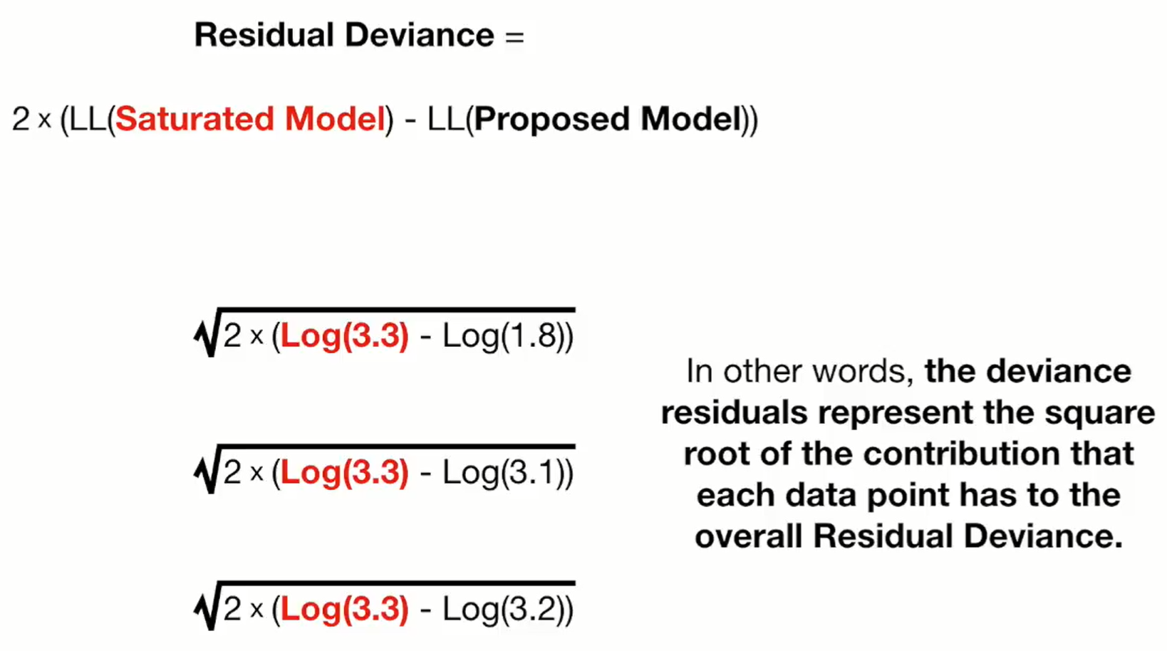
- Top line: “3.3” is the likelihood for a data point in the saturated model and “1.8” is the likelihood for that same data point in the proposed model
- Therefore, squaring each residual and summing them would give you the Residual Deviance for the model.