Causal Inference
Misc
- Notes from
- Packages
- {BCDAG} - Bayesian Structure and Causal Learning of Gaussian Directed Graphs
- {caugi} - A fast and flexible toolbox for building, coercing and analyzing causal graphs
- DAG builder with some unique graphing features. Some graph analysis tests as well.
- {MLCausal} - Provides an end-to-end workflow for estimating average treatment effects in clustered (multilevel) observational data.
- Includes cluster-aware propensity score estimation using fixed effects and Mundlak-style specifications, inverse probability weighting, within-cluster nearest-neighbor matching.
- Has covariate balance diagnostics at both individual and cluster-mean levels, outcome regression with cluster-robust standard errors, propensity score overlap visualization, and tipping-point sensitivity analysis for omitted cluster-level confounding.
- {DAGassist} - Test Robustness with Directed Acyclic Graphs
- Given a ‘dagitty’ DAG object and a model specification, ‘DAGassist’ classifies variables by causal roles, flags problematic controls, and generates a report comparing the original model with minimal and canonical adjustment sets.
- {dagitty} (tool) - A port of the web-based software ‘DAGitty’ for analyzing structural causal models (also known as directed acyclic graphs or DAGs). (See {ggdag})
- {dda} - A collection of tests to analyze the causal direction of dependence in linear models (including interactions)
- Perform Direction Dependence Analysis for variable distributions, residual distributions, and independence properties of predictors and residuals in competing causal models.
- {EconCausal} - Causal Analysis for Macroeconomic Time Series (ECM-MARS, BSTS, Bayesian GLM-AR(1))
- {fastEDM} (Paper, Video, Video)- Implements a series of Empirical Dynamic Modeling tools that can be used for causal analysis of time series data. (Also avaiable in python)
- {fasttreeid} - Determines, for a structural causal model (SCM) whose directed edges form a tree, whether each parameter is unidentifiable, 1-identifiable or 2-identifiable (other cases cannot occur), using a randomized algorithm with provable running time \(O(n^3 log^2 n\))
- {ggdag} - Uses {dagitty} to create and analyze structural causal models (DAGs) and plot them using {ggplot2} and {ggraph} in a consistent and easy manner.
- Also see Confounding >> Example 2
- Edge Types: {ggraph} reference, vignette
- Change color of edges: {ggraph} scales
- {infocausality} (Paper) - Methods for quantifying temporal and spatial causality through information flow, and decomposing it into unique, redundant, and synergistic components. (Seems to be for spatial or time series and not explicitly spatio-temporal)
- {spEDM} - Spatial Empirical Dynamic Modeling
- Resources
- Papers
- A Latent Causal Inference Framework for Ordinal Variables (code)
- Perfect counterfactuals for epidemic simulations (code)
- Cross-Validated Causal Inference: a Modern Method to Combine Experimental and Observational Data (code)
- Complementary strengths of the Neyman-Rubin and graphical causal frameworks
- Specific examples of data-generating mechanisms - such as those involving undirected or deterministic relationships and cycles - where analyses using a directed acyclic graph are challenging, but where the tools from the Neyman-Rubin causal framework are readily applicable.
- Examples of data-generating mechanisms with M-bias, trapdoor variables, and complex front-door structures, where the application of the Neyman-Rubin approach is complicated, but the graphical approach is directly usable.
- Pearl Causal Hierarchy (PCH)
- First Level: Reasons about associations and passively observed data
- Second Level: Investigates the effects of interventions (e.g., determining the effect of a policy change).
- Third Level: Counterfactuals — reasoning about hypothetical situations that would have occurred under different interventions, as opposed to actual events.
- Statistical models measure associations (e.g. linear, non-linear) which is mutual information among the variables
- e.g. wind and leaves moving in a tree (doesn’t answer whether the leaves moving creates the wind or the wind creates leaving moving)
- Causal inference predicts the conseqences after an intervention (i.e. action)
- You must know the direction of causation in order to predict the conseqences of an intervention (unlike measuring associations)
- Answers the question, “What happens if I do this?”
- Causal inference is able to reconstruct unobserved counterfactual outcomes.
- Answers the question, “What happens if I had done something else?”
- Causal assumptions are necessary in order to make causal inferences
- multiple regression does not distinguish causes from confounds
- p-values are not causal statements
- Designed to control type I error rate
- AIC, etc are purely predictive
- Causal Experiment Assumptions
- see tlverse workshop notes and ebook for listing of assumptions and definitions, https://tlverse.org/acic2019-workshop/intro.html#identifiability
- The tlverse Project seeks to use ML models to calculate causal effects. Uses Super Learner ensembling and Targeted Maximum Likelihood Estimation (TMLE) which they call Targeted Learning.
- Ignorability - By randomly assigning treatment, researchers can ensure that the potential outcomes are independent of treatment assignment, so that the average difference in outcomes between the two groups can only be attributable to treatment
- see tlverse workshop notes and ebook for listing of assumptions and definitions, https://tlverse.org/acic2019-workshop/intro.html#identifiability
- Engineering outcome variables using potential adjustment variables does not automatically adjust for those variables in your model
- Notes from There Are No Magic Outcome Variables
- Example
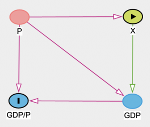
- P is population density
- X is the variable of interest
- GDP and P have been used to create GDP/P
- P influences X and provides a backdoor path to GDP/P, so P must be adjusted for
- Even if P doesn’t influence X, the point is that constructing GDP/P using P doens’t automatically adjust for P
- Randomized experiments remove all paths from the treatment variable, X
.png)
- Adjusting for Z, B, and C can add precision to measurement of the treatment effect since they are causal to Y, but they aren’t necessary to get an unbiased estimate of the treatment effect.
- Table 2 fallacy (Notes from McElreath video, 2022 SR Lecture 6)
- The 2nd table presented in a paper is usually a summary of all the effects of a regression. The fallacy is that the coefficient of each variable is treated as causal.
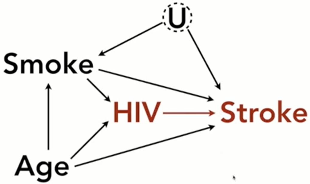
- Example: The effect of HIV on Stroke
- The model is lm(Stroke ~ HIV + Smoke + Age)
- Only the coefficient of the HIV variable should be treated as causal and none of the other adjustment variables (Smoke, Age)
- The effects for Smoke and Age are only partial.
- There are likely unobserved confounding variables, U, on the effect of Smoking on Stroke (e.g. other lifestyle variables).
- Smoke is confounded so it’s causal estimate is biased
- Age is also confounded since Smoke is now a collider and has been conditioned upon. This opens the non-causal path, Age-Smoke-U-Stroke.
- Age-Smoke is frontdoor, but the backdoor path, Smoke-U, also becomes a backdoor path for Age once Smoke is conditioned upon. (aka sub-backdoor path)
- So any open path that contains a backdoor path must also be closed
- The model is lm(Stroke ~ HIV + Smoke + Age)
- Solutions
- Don’t include effect estimates of adjustment variables
- Explicitly interpret each effect estimate according to the causal model
- See 2022 SR at the end of Lecture 6 where McElreath breaks down the interpretation of each adjustment variable estimated effect.
- Causal Forests
- Instead of minimizing prediction error (RFs), data is split in order to maximize the difference across splits in the relationship between an outcome variable and a “treatment” variable. This is intended to uncover how treatment effects vary across a sample.
- Causal forests simply uncover heterogeneity in a causal effect, they do not by themselves make the effect causal. A standard causal forest must assume that the assignment to treatment is exogenous, as it might be in a randomized controlled trial. Some extensions of causal forest may allow for covariate adjustment or for instrumental variables.
- If using causal forest to estimate confidence intervals for the effects, in addition to the effects itself, it is recommended that you increase the number of trees generated considerably.
- Notes from
- Packages
- {grf} - Provides non-parametric methods for heterogeneous treatment effects estimation (optionally using right-censored outcomes, multiple treatment arms or outcomes, or instrumental variables), as well as least-squares regression, quantile regression, and survival regression, all with support for missing covariates.
- Resources
- Synthetic Datasets
- Notes from
- Evaluations of Causal ML methods rely predominantly on synthetic datasets due to the fundamental problem of causal inference: for the same unit, it is impossible to observe the outcome under both conditions: when it has acted and when it has not.
- Despite the advantages of synthetic data (e.g. controlled experiments), the reliance on synthetic data constitutes a major adoption limitation, as such datasets often fail to represent the complexities of real-world scenarios. Its inability to capture unknown unknowns—phenomena or dynamics outside the scope of the data-generating process underscores the importance of complementing synthetic data evaluations with real-world experiments and alternative methodologies to ensure comprehensive and robust assessments
- Principles for Rigorous Causal ML Synthetic Evaluation
- Synthetic data is Necessary for Rigorous Evaluation
- Since real-world datasets cannot provide access to counterfactual outcomes
- Although, synthetic data alone is not necessarily sufficient or the only valid way of evaluating a Causal ML method.
- Semi-synthetic data can introduce a degree of realism that is valuable in certain contexts.
- However, such data also originates from Causal ML generation methods, which must themselves be rigorously evaluated before they can be relied upon.
- Therefore, semi-synthetic data generation methods should first be rigorously evaluated using synthetic data to identify their limitations.
- Synthetic Design Choices Must Be Clearly Stated to Mitigate Unconscious Bias
- Make all experiment design choices transparent, to be clear on the domain of validity of the drawn results.
- Experimental Choices to be Made Transparent
- The set of causal models studied
- The set of causal queries of interest
- The set of training data
- The generation algorithm producing the synthetic causal models, queries, and datasets
- The distribution that the generation algorithm implies on the space of synthetic examples defined by the Choices one, two, and three.
- See Section 4.2 of the paper for an example
- Go Beyond Aggregated Accuracy in the Identification Domain With Comprehensive Experiments
- Methods must also be tested in scenarios that challenge their assumptions, such as shifts in causal structures. Evaluating models both within and beyond their identification domains exposes failure modes and provides insights into their limits under real-world conditions.
- Define large synthetic experimentation spaces, i.e., large sets of causal models and datasets as defined in Principle 1
- Reducing evaluation to accuracy risks ignoring critical dimensions such as robustness, scalability, stability, and interpretability
- Focusing solely on performance metrics can lead to biased evaluations and a misleading perception of progress. By systematically documenting negative results, exploring edge cases, and analyzing failure scenarios, researchers can uncover deeper knowledge that drives theoretical and practical advancements.
- Take a progressive approach to increasing simulation complexity.
- Begin with a simple, intuitive experiment, e.g., a small graph, simple mechanisms, binary variables, sufficient data, and no assumption violations.
- Gradually introduce one new complexity at a time, e.g., hidden confounders, selection bias, small datasets, or mixtures of SCMs.
- For each added complexity, carefully analyze its impact on the method’s performance before adding the next one.
- Additional complexities to consider include the presence of outliers, violation of the ignorability assumption, erroneous causal graph, or adjustment sets
- Methods must also be tested in scenarios that challenge their assumptions, such as shifts in causal structures. Evaluating models both within and beyond their identification domains exposes failure modes and provides insights into their limits under real-world conditions.
- Developing Standardized Evaluation Frameworks to Promote Best Practices
- Benchmarking Platforms for CausalAI
- CauseME is dedicated to causal discovery in time series data
- CausalBench encompasses a broader scope of causal tasks, such as treatment effect estimation.
- These platforms provide pre-coded datasets, models, metrics, and evaluation algorithms, which make evaluation procedures more transparent, fair, and easy to use.
- Neither platform currently includes counterfactual estimation tasks. In addition, information on datasets, particularly (semi-) synthetic ones, lacks sufficient details to comply with Principle 2
- Benchmarking Platforms for CausalAI
- Synthetic data is Necessary for Rigorous Evaluation
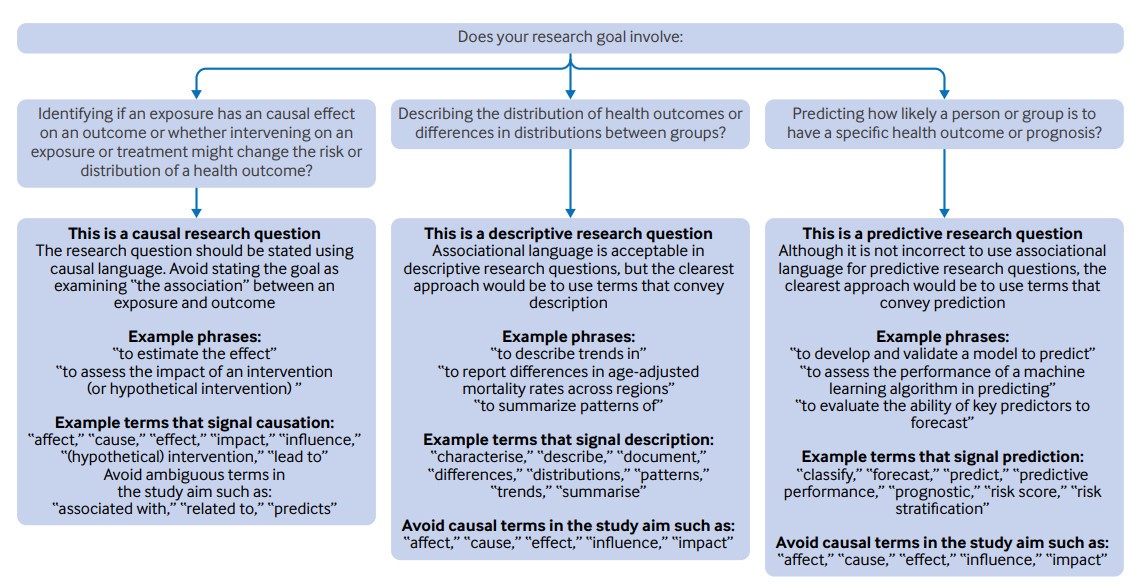
- Appropriate language for results based on the research question (source)
Causal Design
Misc
- Notes from McElreath video
- Overview
- Make a causal model (i.e. DAG)
- Need background information in order to make the causal assumptions represented in the DAG
- DAGs only show whether or not a variable influences another, not how the influence occurs (e.g. DAGs can’t show interactions between variables or whether the association is non-linear)
- Use it to design data collection and statistical procedures
- Make a causal model (i.e. DAG)
- Examples
- Algorithms in Judges’ Hands: Incarceration and Inequity in Broward County, Florida (Also in R >> Documents >> Causal Inference)
- Causal inference, social media, and mental health part 1, part2, part 3
- When trying to determine the relationship (e.g. linear, nonlinear) between variables and remove inconsequential variables, the Double Debiased ML procedure might be useful.
- Double Debiased Machine Learning - basic concepts, links to papers, videos
- EconML (Microsoft) and causalml (Uber) has included the method in their libraries
Creating the DAG
- When trying to infer causal relationships, we should not blindly enter all variables into a regression in order to “control” for them, but think carefully about what the underlying causal DAG could look like. Otherwise, we might induce spurious associations (e.g. confounding such as collider bias).
- Using Domain Knowledge
- Steps:
- Determine two variables of interest (exposure, outcome) that you want to determine if a causal relationship exists and what effect the exposure has.
- Use domain knowledge or prior scholarship to determine the relevant variable and the likely associations between all variables in data
- Create the DAG
- Identify the direct causal path between exposure and outcome
- Identify other explanatory variables and label their directions of influence with each other, the exposure, and the outcome variable
- Consider which variables (especially the exposure and the outcome) have unobserved variables influencing them.
- Steps:
- Causal Discovery
- Misc
- Algorithms that use observational data to fill out a DAG
- Notes from Making Causal Discovery work in real-world business settings
- Packages
- {abn} - Derives a directed acyclic graph (DAG) from empirical data that describes the dependency structure between random variables. The package provides routines for structure learning and parameter estimation of additive Bayesian network models.
- {gadjid} - Graph Adjustment Identification Distances for Causal Graphs
- Method for evaluating causal discovery algorithms. So, probably simulate some data (ground truth) that you’ll eventually want to collect, and test discovery algorithms against it using this package.
- {gCastle} (paper) - Causal Discovery Toolbox
- Provides functionalities of generating data from either simulator or real-world dataset, learning causal structure from the data, and evaluating the learned graph, together with useful practices such as prior knowledge insertion, preliminary neighborhood selection, and post-processing to remove false discoveries
- Markov Equivalence Class - A set of DAGS that are all equally likely.
- Types
- Constraint-based: Starts with a fully connected graph and uses conditional-independence tests to remove edges
- Score-based: Starts with a disconnected graph and iteratively adds new edges computing a score to assess how well the last iteration modeled the distribution
- Function-based: Leverages information about functional forms and properties of distributions to identify causal directions
- Gradient-based: Essentially a score-based method, but treated as a continually optimized task.
- Assumptions
- Causal Markov Condition: Each variable is conditionally independent of its non-descendants, given its direct causes.
- This tells us that if we know the causes of a variable, we don’t gain any additional power by knowing the variables that are not directly influenced by those causes. This fundamental assumption simplifies the modelling of causal relationships enabling us to make causal inferences.
- Causal Faithfulness: If statistical independence holds in the data, then there is no direct causal relationships between the corresponding variables.
- Testing this assumption is challenging and violations may indicate model misspecification or missing variables.
- Causal Sufficiency: All the variables included are sufficient to make causal claims about the variables of interest.
- In other words, we need all confounders of the variables included to be observed. Testing this assumption involves sensitivity analysis which assesses the impact of potentially unobserved confounders.
- Acyclicity: No cycles in the graph.
- Causal Markov Condition: Each variable is conditionally independent of its non-descendants, given its direct causes.
- PC (Peter and Clark) Algorithm
- Constraint-based algorithm that uses independence tests
- See Association, General >> Hoeffding’s D, KCI test, dcor for continuous variables
- See mixed types and dcor for mixed variable type comparisons
- KCI has a conditional test and maybe the Regression kernel can handle mixed variable types.
- See Discrete Analysis notebook for Chi-Square, Likelihood Ratio, and Fisher’s Exact tests for categorical variables
- Fisher’s may have a conditional test and binning a continuous variable may make a potential option for mixed variable types.
- See Association, General >> Hoeffding’s D, KCI test, dcor for continuous variables
- Steps
- Start with a fully connected graph. Then use conditional independence tests to remove edges and identify the undirected causal graph (nodes linked but with no direction).
- Share this undirected graph with domain experts and use them to help add causal directions between the nodes and complete the DAG.
- Constraint-based algorithm that uses independence tests
- Misc
Analysis Steps
- Analyze the DAG
- Identify colliders and use d-separation to determine conditional independencies
- Identify additional paths (backdoor paths, sub-backdoor paths) between exposure and outcome
- Use the backdoor criterion to determine the set of variables that need to be adjusted for in order to block all backdoor paths with only the direct causal path remaining open.
- Add additional adjustment variables that are causal to the outcome variable (but don’t confound the treatment effect) in order to add precision to the estimate of the treatment effect
- Create simulated data that fits the DAG (i.e. a generative model)
- Perform statistical analysis (i.e. SCMs) on the simulated data to make sure you can measure the causal effect.
- Design experiment and collect the data
- Run the statistical analysis on the collected data and calculate the average causal effect (ACE) under the assumptions that your DAG and model specifications are correct.
- Based on your results, revise the DAG and SCM as necessary and repeat as necessary
Bad Adjustment Variables
- Code and more details included in 2022 SR, Lecture 6
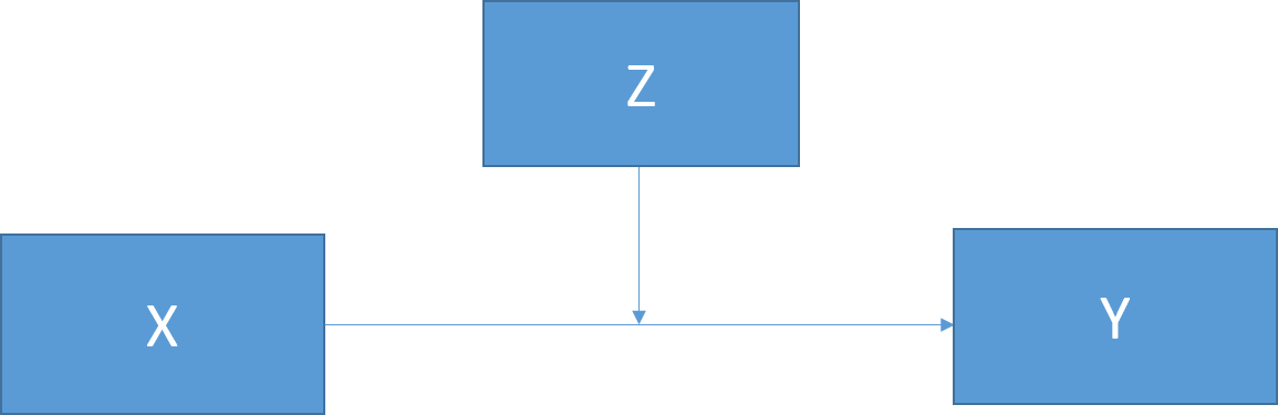
- For all examples, Z is the adjustment variable that’s being considered; X is the treatment and Y is the outcome
- In each scenario, including Z produces a biased estimate of X, so the correct model is Y ~ X.
- M-bias
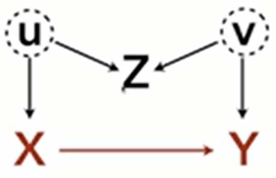
- Z doesn’t have a direct causal influence on the either X or Y, but when it’s conditioned upon it becomes a collider due to unobserved confounds that have a direct causal influence on X and Y.
- Common issue in Political Science and network analysis
- Example
- Y: Health of Person 2
- X: Health of Person 1
- Z: Friendship status
- Pre-treatment variable (tend to be open to collider paths) since they could be friends before the exposure
- U: Hobbies of Person 1
- V: Hobbies of Person 2
- Post-Treatment Bias
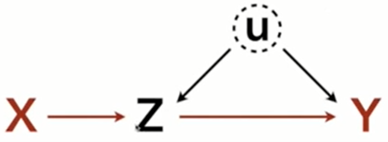
- Z is a mediator and conditioning upon Z blocks the path from X to Y, but opens the backdoor path through the unobserved confound, U.
- Common in medical studies
- Example
- Y: Lifespan
- X: Win Lottery
- Z: Happiness
- U: Contextual Confounds
- Selection Bias
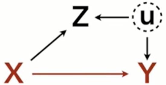
- Same as collider bias
- This version adds an unobserved confounder
- If the experimenter doesn’t take into account or know about U, then the dag they’d draw would include an arrow from Z to Y (without U). They’d condition on Z to try to block that path from Z to Y, not knowing it’s actually a collider, which would actually open a path from Z to U to Y
- Example
- Y: Income
- X: Education
- Z: Values
- U: Family
- Same as collider bias
- Case-Control Bias
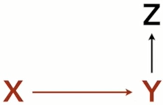
- Z is a descendent. Since Z has information about Y, conditioning on it will narrow the variation of Y and distort the measured effect of X.
- Also see Association >> Single Path DAGs >> Descendent
- Example
- Y: Occupation
- X: Education
- Z: Income
- Precision Parasite
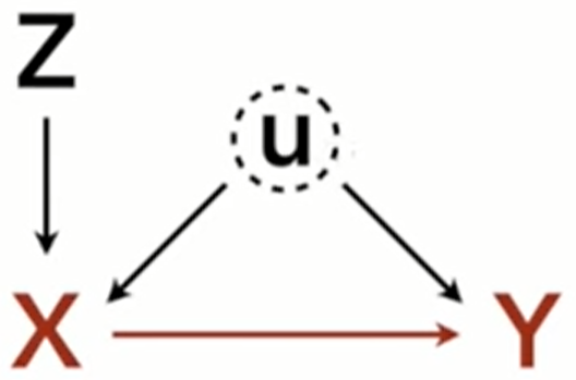
- 2 versions: with and without U
- Without U, conditioning on Z removes variation from X and lessens (but doesn’t bias) the precision of the estimated effect of X on Y (i.e. inflated std.error)
- With U, the effect of X is biased and that bias is amplified when Z is included.
- 2 versions: with and without U
- Peer Bias
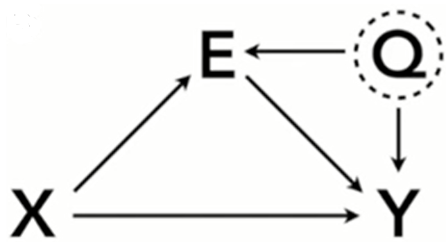
- Classic DAG of the Berkley Admission-Race-Department study
- Also see Structural Causal Models >> Example (Bayesian Peer Bias)
- X is race, E is department, Q is unobserved (e.g. student quality), Y is Admission
- Department cannot be conditioned upon because it’s a collider with Q and would bias the estimate of X through a sub-backdoor path, X-E-Q-Y
- Only the total effect of X on Y can be estimated (Y ~ X) since E cannot be conditioned upon but that’s not interesting and maybe not precise
Terms
- Average Causal Efffect (ACE) - average population effect that’s calculated from an intervention (see Counterfactual definition for info on Individual Causal Effects)
- If X is binary, then
 is the average causal effect (see Simpson’s Paradox example)
- Calculated from a contingency table
- Also,

- This looks like the interpretation of the slope in a regression model.
- If X is binary, then
- Backdoor Criterion - A valid causal estimate is available if it is possible to condition on variables such that all backdoor paths are closed
- Given two nodes, X and Y, an adjustment set, L, fulfills the backdoor criterion if
- no member in L is a descendant of X and
- members in L block all backdoor paths (“shutting the backdoor”) between X and Y.
- Adjusting for L thus yields the causal effect of X→Y.
- After executing an intervention, the conditional distribution in the observational DAG (seeing) will correspond to the interventional distribution (doing) when blocking the spurious path. (see Simpson’s Paradox example)
- Given two nodes, X and Y, an adjustment set, L, fulfills the backdoor criterion if
- Backdoor Path - A non-causal path that enters a causal variable in a DAG rather than exits it.
- e.g. the path that connects a collider to a causal variable points from the collider to the causal variable
- Sub-backdoor Path - this path begins with a frontdoor path but through conditioning on a variable, it opens a connecting backdoor path which biases the treatment effect
- see Misc >> Table 1 Fallacy and Causal Design >> Bad Adjustment Variables >> Peer Bias
- The causal effect is the distribution of Y when we change x, averaged over the distributions of the adjustment variables (Z)

- Causal Hierarchy (lowest to highest)
- Association
- associated action: Seeing - observational; observing the value of Y when X = x
 , observational distribution; What values Y would likely take on if X happened to equal x.
- associated action: Seeing - observational; observing the value of Y when X = x
- Intervention
- associated action (do-Calculus): Doing - experimental; observing the value of Y after setting X = x
 , interventional distribution; What values Y would likely take on if X would be set to x.
- Using the do operator allows us to make inferences about the population but not individuals.
- do(X) means to cut all of the backdoor paths into X, as if we did a manipulative experiment. The do-operator changes the graph, closing the backdoors.
- The do-operator defines a causal relationship, because Pr(Y|do(X)) tells us the expected result of manipulating X on Y, given a causal graph.
- We might say that some variable X is a cause of Y when Pr(Y|do(X)) > Pr(Y|do(not-X)).
- (makes more sense to me with a binary outcome, Pr(Y = 1|do(X), but maybe Y as a continuous variable can be defined a subset. …I dunno)
- We might say that some variable X is a cause of Y when Pr(Y|do(X)) > Pr(Y|do(not-X)).
- The ordinary conditional probability comparison, Pr(Y|X) > Pr(Y|not-X), is not the same. It does not close the backdoor.
- Note that what the do-operator gives you is not just the direct causal effect. It is the total causal effect through all forward paths.
- To get a direct causal effect, you might have to close more backdoors.
- The do-operator can also be used to derive causal inference strategies even when some backdoors cannot be closed.
- associated action (do-Calculus): Doing - experimental; observing the value of Y after setting X = x
- Counterfactual
- associated action: Imagining - what would be the outcome if the alternative would’ve happened.
- Individual Causal Effects can be calculated but it requires stronger assumptions and deeper understanding of the causal mechanisms
- Need to research this part further.
- If the underlying SCM is linear then the ICE = ACE.
- Association
- A collider along a path blocks that path. However, conditioning on a collider (or any of its descendants) unblocks that path
- When a collider is conditioned upon, the change in the association between the two nodes it separates is called collider bias.
- e.g. if Z is a collider between X and Y, conditioning upon Z will induce an association between X and Y.
- When a collider is conditioned upon, the change in the association between the two nodes it separates is called collider bias.
- A conditioning set, \(L\), is the set of nodes we condition on (it can be empty).
- Confounding is the situation where a (possibly unobserved) common cause obscures the causal relationship between two or more variables.
- There is more than one causal path between two nodes.
- A causal effect of X on Y is confounded if

- Collider bias is a type of confounding. When a collider is controlled for, a second (or more) path opens, and the effect is confounded
- X and Y are d-separated by [L if conditioning on all members in [L blocks all paths between the nodes, X and Y.
- Tool for checking the conditional independencies which are visualized in DAGs.
- A descendant is a node connected to a parent node by that parent node’s outgoing arrow.
- Frontdoor Adjustment - In a causal chain with three nodes X→Z→Y, we can estimate the effect of X on Y indirectly by combining two distinct quantities: (Useful for when unobserved confounders prevent direct causal estimation)
- The estimate of the effect of X on Z, P(Z|do(X))
- The estimate of the effect of Z on Y, P(Y|do(Z), X)
- Frontdoor Path - a path that exits a causal variable in a DAG rather than enters it.
- e.g. the path that connects a causal variable, X, to an outcome variable, Y, has an arrow that points from X to Y.
- Markov Equivalence - A set of DAGs, each with the same conditional independencies
- Mediation Analysis - seeks to identify and explain the mechanism or process that underlies an observed relationship between an independent variable and a dependent variable via the inclusion of a third hypothetical variable, known as a mediator variable (z-variable in the DAGs of “pipes” below)
- Including a mediator and the independent variable in a regression will result in the independent variable not being signficant and the mediator being significant.
- Moderation Analysis - Like mediation analysis, it allows you to test for the influence of a third variable, Z, on the relationship between variables X and Y, but rather than testing a causal link between these other variables, moderation tests for when or under what conditions an effect occurs.
- A node is a parent of another node if it has an outgoing arrow to that node
- A path from X to Y is a sequence of nodes and edges such that the start and end nodes are X and Y, respectively.
- Residual Confounding occurs when a confounding variable is measured imperfectly or with some error and the adjustment using this imperfect measure does not completely remove the effect of the confounding variable.
- Example: Women who smoke during pregnancy have a decreased risk of having a Down syndrome birth.
- This is puzzling, as smoking is not often thought of as a good thing to do. Should we ask women to start smoking during pregnancy?
- It turns out that there is a relationship between age and smoking during pregnancy, with younger women being more likely to indulge in this bad habit. Younger women are also less likely to give birth to a child with Down syndrome. When you adjust the model relating smoking and Down syndrome for the important covariate of age, then the effect of smoking disappears. But when you make the adjustment using a binary variable (age<35 years, age >=35 years), the protective effect of smoking appears to remain.
- Example: Women who smoke during pregnancy have a decreased risk of having a Down syndrome birth.
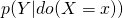
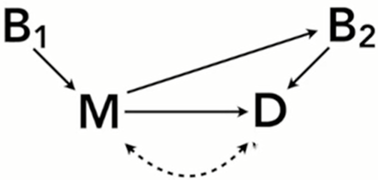
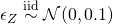
- Structural Causal Models (SCMs) - relate causal and probabilistic statements; each equation is a causal statement
- “:=” is the assignment operator
- X is a direct cause of Y which it influences through the function f( )
- where f is a statistical model
- The noise variables, ϵX and ϵY, are assumed to be independent.
- There are Stochastic and Deterministic SCMs. Deterministic SCMs presented in article.
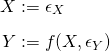
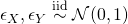
Association
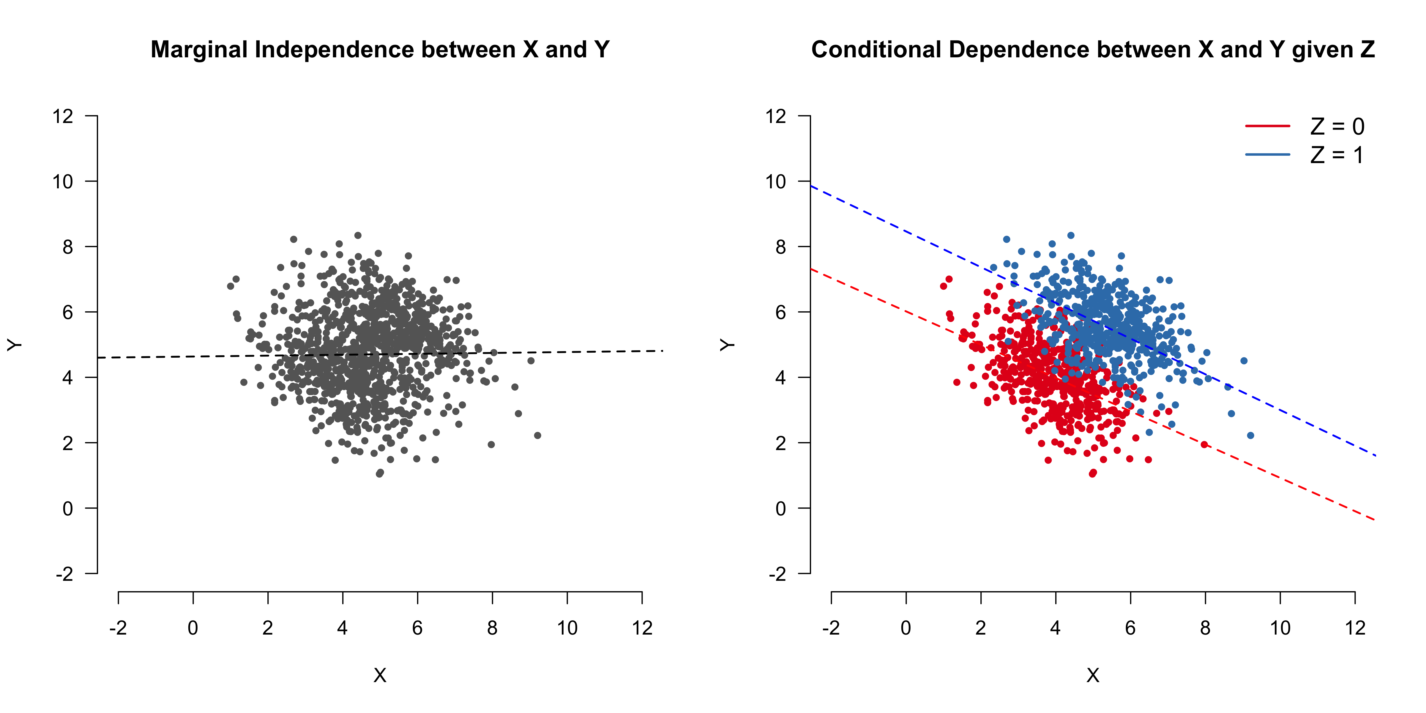
- Far left: lm(Y ~ X); X and Y show a linear correlation when Z is NOT conditioned upon
- Left: lm(Y ~ X + Z); X and Y show NO linear correlation when Z is conditioned upon
- Right: lm(Y ~ X); X and Y show NO linear correlation when Z is NOT conditioned upon
- Far Right: lm(Y ~ X + Z); X and Y show a linear correlation when Z is conditioned upon
Single path DAGs
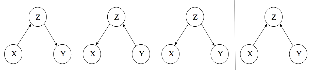
- For each of these DAGs, Z would be the only member of the conditioning set.
- The first 3 DAGs represent the scatter plots above
- Z only blocks the path between X and Y when it’s conditioned upon.
- X and Y are associated (e.g. linear correlation, mutual information, etc.) when Z is ignored
- Conditioning on Z results in X and Y no longer being associated (i.e. conditional independence)
- The first and second DAGs are elemental confounds or relations called “Pipes.”
- The left one
- In general, DO NOT add these variables to your model
- These paths are causal so they shouldn’t be blocked
- If your goal isn’t causal inference, then adding these variables might provide predictive information
- e.g. If there was a causal arrow from X to Y, the far left DAG would NOT have a backdoor path and therefore Z would not be conditioned upon to block the path, X-Z-Y
- The path from X to Z is a frontdoor path since the arrow exits X.
- Sometimes you DO condition on these variables
- During mediation analysis, you condition on these variables as part of the process to determine how much of the effect goes through Z.
- The mediation path can have an important interpretation depending on your research question
- e.g. Indirect Descrimination
- i.e. Some of effect of gender (independent) on being admitted (dependent) has to do with the student’s choice of department (mediator). Some departments are harder to get into because they’re more popular and there are few spots.
- Mediation Analysis can help determine how much of the effect is direct discrimination and indirect discrimination
- See Statistical Rethinking >> Chapter 11 >> Conclusion of Berkeley Admissions example
- also Lecture 9 2022 video
- e.g. Indirect Descrimination
- In general, DO NOT add these variables to your model
- The right one is a backdoor path and should be conditioned on.
- Everything you can learn about Y from X (or vice versa) happens through Z, therefore learning about X separately provides no additional information
- Z is traditionally labelled a mediator
- The left one
- The third DAG is an elemental confound or relation called a “Fork.”
- In general, add these variables to your model
- These are backdoor paths and are NOT causal
- X and Y have a common cause in Z and some of the mutual information about Z they each contain, overlaps, and creates an association (when Z isn’t conditioned upon).
- Z only blocks the path between X and Y when it’s conditioned upon.
- The fourth DAG is an elemental confound or relation called a “Collider.”
.png)
- In general, do NOT add these variables to your model
- Z blocks the path between X and Y unless conditioned upon.
- An association between X and Y is induced by conditioning on Z, lm(Y ~ X + Z)
- X and Y are independent causes of Z. Z contains information about both X and Y, but X doesn’t contain any information about Y and vice versa.
- A small X and a sufficiently large Y (and vice versa) can produce a Z = 1. So X and Y have compensatory relationship in causing Z.
- i.e. For a given value of Z, learning something about X tells us what Y might have been.
- The last elemental confound or relation is called a “Descendent.”
.png)
- Conditioning on a descendent variable, D, is like conditioning on the variable, Z itself, but weaker. A descendent is a variable influenced by another variable.
- Controlling for D will also control, to a lesser extent, for Z. The reason is that D has some information about Z.
- This will (partially) open the path from X to Y, because Z is a collider.
- See Confounding >> Example 2
- The same holds for non-colliders. If you condition on a descendent of Z in the pipe, it’ll still be like (weakly) closing the pipe.
- This will (partially) open the path from X to Y, because Z is a collider.
Dual path DAGs
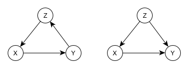
- Causal paths do not flow against arrows but associations can.
- Two examples of DAGs representing confounding
- These are the 2 middle DAGs above with an additional path from X to Y
- If Z is NOT conditioned on (i.e. top path is not blocked), then the causal effect of X on Y would be confounded.
- The paths from X to Y:
- The path through Z matches the first DAG.
- Therefore X and Y are conditionally independent given Z.
- The path through W matches the fourth DAG
- Therefore X and Y are conditionally dependent given W.
- The path through Z matches the first DAG.
- The path through W (collider) is blocked unless W is conditioned upon
- The path through Z is open unless Z is conditioned upon
- If Z and W are conditioned upon, then the path between X and Y is open through W and an association is present.
Intervention
- Since actual interventions are usually unfeasible, we want to be able to determine causality with observational data. This requires two assumptions:
- The intervention occurs locally. Which means that only the variable we target is the one that receives the intervention.
- The mechanism by which variables interact do not change through interventions; that is, the mechanism by which a cause brings about its effects does not change whether this occurs naturally or by intervention
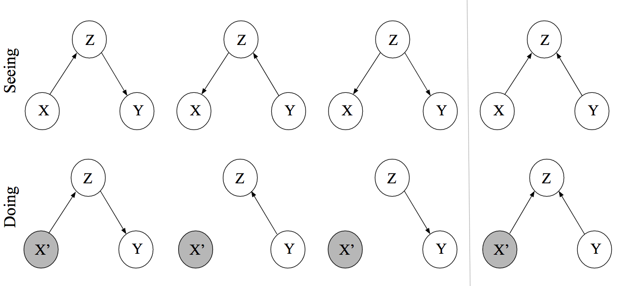
- The Doing row of DAGs (aka manipulated DAGs) represents setting X = x
- For DAGs 1 and 4, Y is still affected
- Moving from seeing to doing didn’t change anything

- Moving from seeing to doing didn’t change anything
- For DAGs 2 and 3, Y is now UNaffected
- Using the assumptions and some mathematical manipulation (See article for details):
-
- Thus, the interventional distribution we care about is equal to the (observational) conditional distribution of Y given X when we adjust for Z
- Using the assumptions and some mathematical manipulation (See article for details):
- For DAGs 1 and 4, Y is still affected
- The rule: After an intervention, incoming arrows are cut from the node where the intervention took place.
Confounding
The backdoor criterion tells us which variable we need to adjust for in order to for our model to yield a causal relationship between two variables (i.e. graphically, nodes)
- Blocks all spurious, that is, non-causal paths between X and Y.
- Leaves all directed paths from X to Y unblocked
- Creates no spurious paths
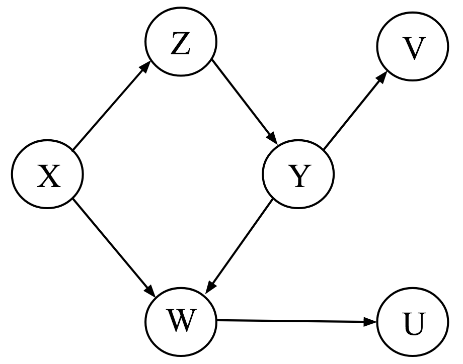
Example 1
- Causal effect of Z on U is confounded by X because in addition to the legitimate causal path Z→Y→W→U, there is also an unblocked path Z←X→W→U which confounds the causal effect
- Since X’s arrow enters the causal variable of interest, Z, it’s arrow is a backdoor path and needs to be blocked/closed
- There are some descendant nodes that make the confounding a little difficult to parse out, but this graph is essentially
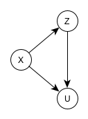
- which is the same as the second example DAG for confounding in the Association section
- The backdoor criterion would have us condition on X, which blocks the spurious path and renders the causal effect of Z on U unconfounded.
- The reduced, confounding DAG above is the same as the third DAG (without the path from Z to U) in the Association section. Conditioning on Z in that example blocked the path between X and Y, so it makes sense that conditioning on X in the reduced DAG would block the Z to X to U path. And therefore, the Z←X→W→U would also be blocked in the complete DAG.
- Note that conditioning on W would also block this spurious path; however, it would also block the causal path, Z→Y→W→U.
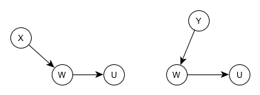
If we breakdown the complete DAG into the modular components involving W, we can see these are the same as the first example DAG in the Association section.
W is also collider for X and Y, but I don’t think that has any bearing when discussing the causal effect of Z on U.
- Causal effect of Z on U is confounded by X because in addition to the legitimate causal path Z→Y→W→U, there is also an unblocked path Z←X→W→U which confounds the causal effect
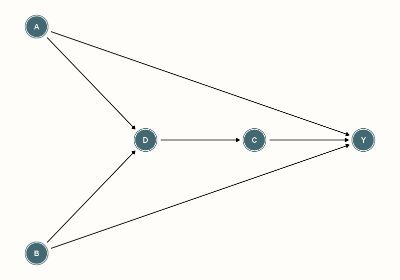
Example 2: Estimate the direct and total effects from A to Y (source)
Set-Up
library(ggdag); library(ggplot2)

notebook_colors <- unname(swatches::read_ase(here::here("palettes/Forest Floor.ase")))

theme_dag_notebook <- function(...){
  ggdag::theme_dag() +
    theme(
      panel.background = element_rect(fill='#FFFDF9FF',
                                      color = NA),
      panel.border = element_blank(),
      panel.grid.minor = element_blank(),
      plot.background = element_rect(fill='#FFFDF9FF',
                                     color = NA),
      legend.background = element_rect(color = NA,
                                       fill='#FFFDF9FF'),
      legend.box.background = element_rect(fill='#FFFDF9FF',
                                           color = NA),
      ...
  )
}
da_dag <- dagify( Y ~ A + B + C, D ~ A + B, C ~ D, outcome = "Y", exposure = "A" ) |> tidy_dagitty(layout = "sugiyama") da_dag |> ggplot(aes( x = -.data$y, y = -.data$x, xend = -.data$yend, yend = -.data$xend) ) + geom_dag_node(color = notebook_colors[[6]]) + geom_dag_edges() + geom_dag_text() + theme_dag_notebook()- Note: Set-up code is folded above
- layout = “sugiyama” is especially designed for DAGs
- DAGS go from top to bottom by default. By interchanging x and y, xend and yend, along with adding negative signs, you able to make a DAG that flows from left to right.
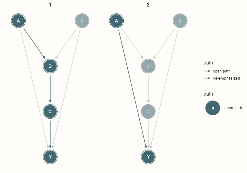
ggdag_paths(da_dag, text = TRUE, shadow = TRUE) + geom_dag_node(color = notebook_colors[[6]]) + geom_dag_text(color = "white") + ggraph::scale_edge_color_manual(values = notebook_colors[[6]], labels = c("open path", "de-emphasized")) + theme_dag_notebook()- There are two direct paths from A to Y and no backdoor paths
- shadow = TRUE includes the de-emphasized paths so you can still see the whole DAG
Direct Effect
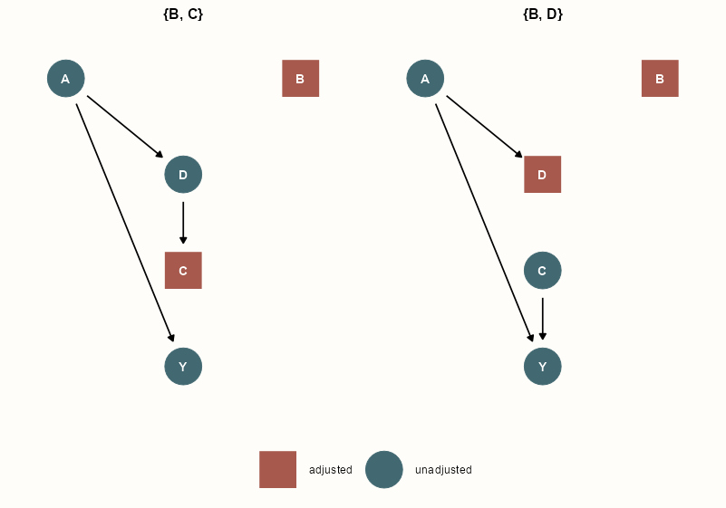
dagify( Y ~ A + B + C, D ~ A + B, D ~ D ) |> dagitty::adjustmentSets( outcome = "Y", exposure = "A", effect = "direct" ) #> { B, C } #> { B, D } ggdag_adjustment_set(da_dag, effect = "direct", node_size = 14) + scale_color_discrete(palette = notebook_colors[c(5,6)]) + theme_dag_notebook( legend.title = element_blank(), legend.position = "bottom" )- To estimate A –direct–> Y, must also adjust for B and (C or D).
- If you adjust for C, it partly opens collider D, so non-causal path D <– B –> Y is opened. Therefore, B needs to adjusted for as well.
- Easy to forget about descendants partly opening parents. Sneaky colliders.
Total Effect
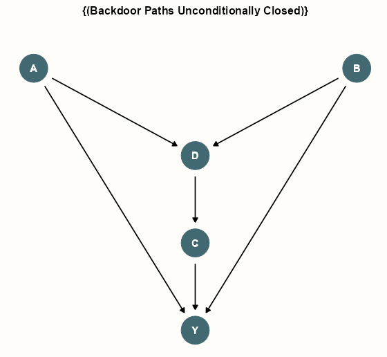
dagify( Y ~ A + B + C, D ~ A + B, D ~ D ) |> dagitty::adjustmentSets( outcome = "Y", exposure = "A", effect = "total" ) #> {} ggdag_adjustment_set(da_dag, effect = "total", node_size = 14) + scale_color_manual(values = notebook_colors[6]) + geom_dag_text(color = "white") + theme_dag_notebook( legend.position = "none" )- There is no additional adjustment needed to estimate the total effect of A on Y. (i.e. just fit Y ~ A)
Application: Simpson’s Paradox Example
Sex as the adjustment variable
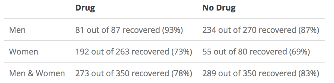
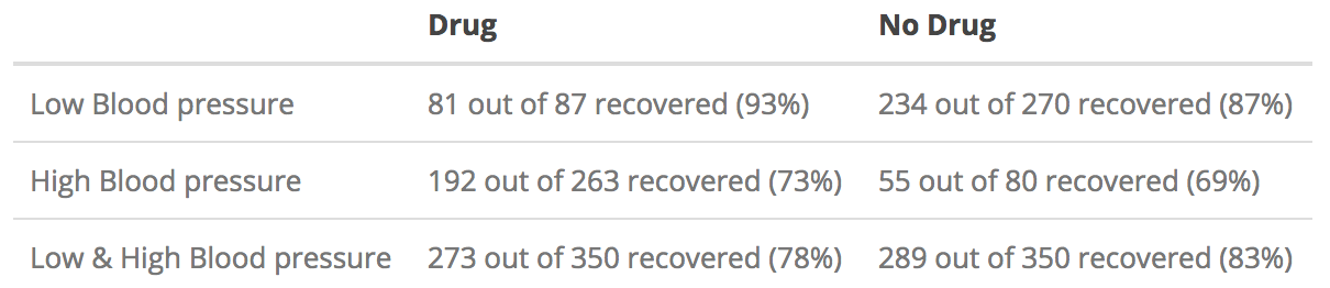
- Patients CHOOSE whether or not to take a drug to cure some disease.
- Men choosing to take the drug recover at a higher percentage that those that didn’t
- Women choosing to take the drug recover at a higher percentage that those that didn’t
- But overall, those that chose to take the drug recovered at a lower percentage than those that didn’t.
- So should a doctor prescribe the drug or not?
- Suppose we know that women are more likely to take the drug, that being a woman has an effect on recovery more generally, and that the drug has an effect on recovery.
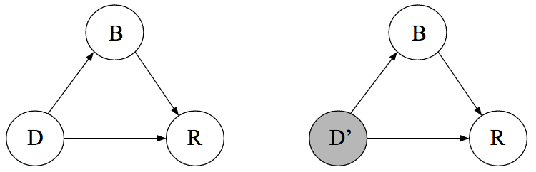
- Create DAGs
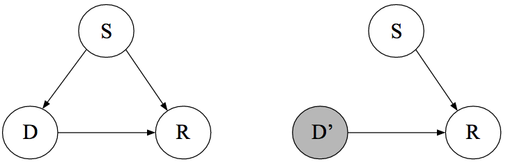
- S=1 as being female,
- D=1 as having chosen to take the drug
- R=1 as having recovered
- The right DAG indicates either forcing everyone to either take the drug or not take the drug
- Notice that
 therefore our calculated effect will be confounded.
- Backdoor criterion says the manipulated DAG (right) will correspond to the observational DAG (left) if we condition on Sex.

Use intervention formula from Intervention section
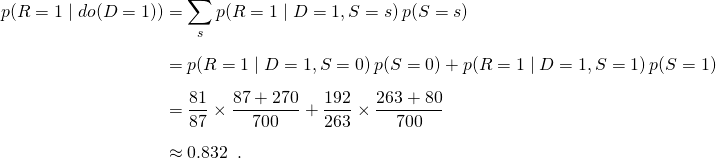
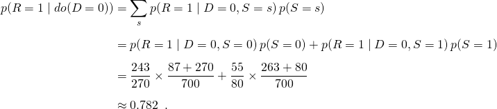
Average Causal Effect = 0.832 - 0.782 = 0.050. So the drug has a positive effect on average.
Blood Pressure as the adjustment variable
- Blood Pressure instead of sex is used as the adjustment. Blood Pressure is a post-treatment variable.
- Relatively same observations as before. High or Low Blood Pressure with the drug produces better results than those that chose not to take the drug. Yet overall, those that chose the drug recovered at a lower percentage.
- Since Blood Pressure (B) is post-treatment, it has no effect on whether the patient takes the drug or not (D).
- Taking or not taking the drug (D) has an indirect effect on recovery (R) through Blood Pressure (B) along with a direct effect.
 so our calculated effect will be unconfounded.
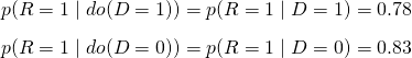
- So with BP as the adjustment variable, the drug now has a small, negative effect (harmful), 0.78 - 0.83 = -0.05
The unconfounded, average causal effect for the population is negative, therefore the doctor should NOT prescribe the drug.
Structural Causal Models (SCMs)
- You add additional assumptions to your DAG to derive a causal estimator
- “Full Luxury” Bayesian approach
- “Full Luxury” is just a term coined by McElreath; it’s just a bayesian model but bayesian models can fully model a DAG where standard regression approachs can fail (see examples)
- No other approach will find something that the bayesian approach doesn’t
- Main disadvantage is that it can be computationally intensive (same with all baysian models)
- Provides ways to add “causes” for missingness and measurement error
- Example (2 Moms)
- Notes from McElreath video
- Hypothesis: a mother’s family size is causal to her daughter’s family size
- Truth: no relationship
- Variables:
- M - Mother’s family size (i.e. number of children the birth)
- D - Daughter’s family size
- B1 - Mother’s birth order; binary, first born or not
- B2 - Daughters’ birth order; binary, first born or not
- U - unobserved confounds (shown as curved dotted line)
- Unobserved confounds (economic status, education, cultural background, etc.) are causal to both Mother and Daughter (curved dotted line) which makes regression, D ~ M, impossible
- See Baysian Two Moms example below for results of a typical regression
- Still possible to calculate the effect of M on D with SCMs
- Unobserved confounds (economic status, education, cultural background, etc.) are causal to both Mother and Daughter (curved dotted line) which makes regression, D ~ M, impossible
- Assumptions: Relationships are linear (i.e. linear system)
- Causal Effects
.png)
- We want m which is the causal effect of M on D
- Assumes causal effect of birth order is the same on mother and daughter
- Aside: There is no arrow/coefficient from M to B2 because it’s not germane to the calculation of m
- Calculate linear effect (i.e. regression coefficient) without a regression model using a linear system of equations
- Note: a regression coefficent, β = cov(X,Y) / var(X)
- We can’t calculate the covariance of M and D directly because it depends on unobserved confounders but we can calculate the covariance between B1 and D and use that to get m.
- The covariance for each path is the product of the path coefficients and the variance of the originating causal variable.
- Path B1 → M: cov(B1, M) = b*var(B1)
- Path B1 → D: cov(B1, D) = b*m*var(B1)
- 2 equations and 2 unknowns, m and b
- Solve for b in the first equation, substitute b into the second equation, and solve for m
- m = cov(B1, D) / cov(B1, M)
- Still need an uncertainty of this value (e.g. bootstrap)
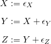
- Example (Bayesian 2 Moms)
- See previous example for link, hypothesis, and definition of the variables
.png)
- Functions (right side)
- Each variable’s function’s inputs are variables that are causal influences (i.e. have arrows pointing at the particular variable
- e.g. M has two arrows pointing at it in the DAG: B1 and u
- Each variable’s function’s inputs are variables that are causal influences (i.e. have arrows pointing at the particular variable
- Code
- The assumption is that this is a lineary system, so M and D have Normal distributions for their functions with means as linear regression equations
- B1 and B2 are binary so they get bernoulli distributions
- U gets a standard normal prior
- Aside: evidently this is a typical prior for latent variables in psychology
- p, intercepts, sd, k get typical priors for bayesian regressions
- Results
.png)
- Truth: no effect
- 1st 3 lm models shows how the unobserved confound biases the estimate when using a typical regression model to estimate the causal effect
- Including B2 adds precision to the biased estimate since it is causal to the outcome D while adding B1 increases the bias
- Bayesian model isn’t fooled because U is specified as an input to the functions for M and D
- Interpretation: There is no reliable estimate of an effect. The most likely effect is a moderately positive one but it could also be negative.
- Adding more simulated data to this example will move the point estimate towards zero
- See previous example for link, hypothesis, and definition of the variables
- Example (Bayesian Peer Bias)
- Also see Causal Design >> Bad Adjustment Variables >> Peer Bias
- Hypothesis: racial discrimination in acceptance of applicatioon to Berkeley grad schools
- Truth: moderate negative effect, -0.8
- Variables:
- X is race, E is department, Q is an unobserved confound (latent variable: student quality), Y is binary; Admission/No Admission
- R1 and R2 are proxy variables for Q (e.g. test scores, lab work, extracurriculars, etc.)
- Assumptions: System is linear
- DAG and Code
.png)
- XX is the race variable with X as the coefficient in the code
- This code uses his {rethinking} package so some of this syntax is unfamiliar
- R1 and R2 are shown in the DAG to be influenced by student quality, Q
- Every prior is normal except for Q’s coefficient
- XX is the race variable with X as the coefficient in the code
- Results
.png)
- Truth: -0.8
- 1st 3 glm models shows how the unobserved confound, Q, biases the estimate when using a typical logistic regression model to estimate the causal effect
- Bayesian model isn’t fooled because Q is specified as an input to the function for Y
- Interpretation: There is a reliably negative effect (no 0 in the CI). The most likely effect is a moderately negative one.
- Not quite equal to the truth but reliably negative and the point estimate is closer than the glms
- Example
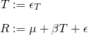
- Assumptions: Relationships between variables are linear and error terms are independent
- Equations
 ,
, 
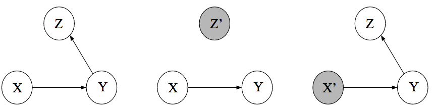
- DAG 1 (left) shows the association DAG which represents the SCM
- manipulated DAG 1 (middle) shows intervention where z is set to a constant
- incoming causal arrows get cutoff the intervening variable
- manipulated DAG 1 (right) shows intervention where x is set to a constant
- Simulation of the SCM (n = 1000) (code in article)
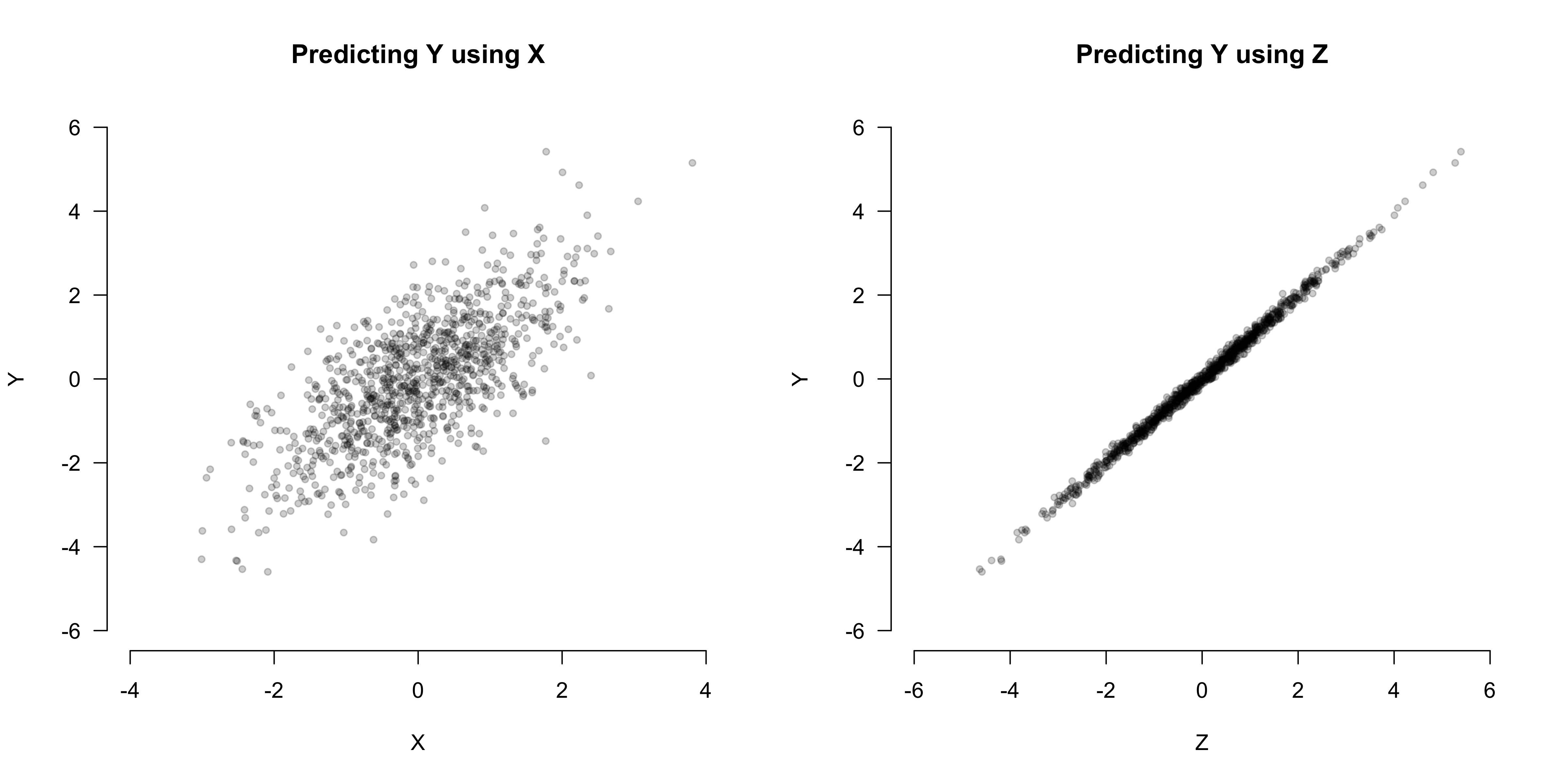
- Z is more predictive of Y than X
- Simulate interventions (code in article)
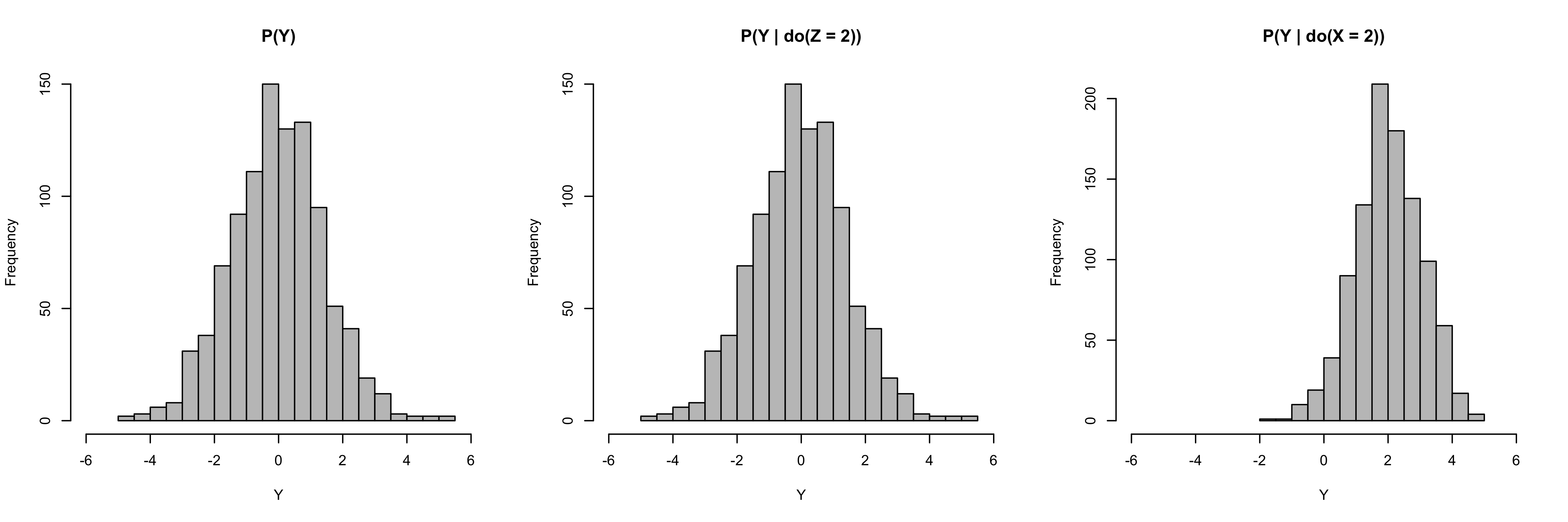
- Left - histogram of SCM for Y without an intervention
- Middle - Intervention on Z
- confirms the DAG which shows no effect on Y and Z is not causal
- Right - intervention on X
- confirms the DAG which shows an intervention on X produces an effect on Y and X is causal
- Average Causal Effect (ACE) can be determined by subtracting the expected values of interventions where X = x +1 and X = x
Counterfactuals
- Example(code in article): Test whether Grandma’s home remedy can speed recovery time for the common cold
- SCM
- T is 1/0, i.e. whether patient receives Grandma’s treatment, with p = 0.5;
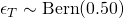
- R is recovery time
- μ is the intercept
- β is the average causal effect, since
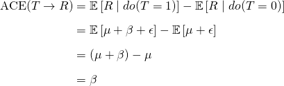
- where

- where
- T is 1/0, i.e. whether patient receives Grandma’s treatment, with p = 0.5;
- From fitting the model, we find μ = 7, β = -2, Τ = 0, ε1 = 0.78
- Therefore, the Individual Causal Effect for patient 1
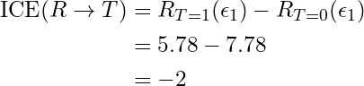
- Just plug and chug where we substitute T = 1 into the SCM and we already have the T = 0 part from the model
- Therefore, the Individual Causal Effect for patient 1
- In this case, the SCM is linear, so the ICE = ACE.
- SCM
Mediation Analysis
.png)
Figure
- c’ is the direct effect of X on the outcome after the indirect path has been removed (i.e. conditioned upon, outcome ~ X + mediator)
- c is the to total effect (outcome ~ X)
- c - c’ equals the indirect effect
- See definitions below
Allows you to test for the influence of a third variable, the mediator, on the relationship between (i.e. effect of) the treatment variable, X, and the Outcome variable, Y. You’re determining how much of X’s effect on Y goes through the mediator.
The goal of studies conducting mediation analyses, particularly in health research, is often to understand how hypothetical interventions targeting mediators might counter exposure effects in order to guide future treatment and policy decisions as well as intervention development.
Misc
- Notes from: Mediation Models
- Overview of packages (Aug 2020)
.png)
- {brms} very flexible in terms of models. You’ll just have to calculate the effects by hand unless some outside package (e.g. sjstats) takes a brms model and does it for you.
- See below for formulas. {mediation} papers should have other formulas for other types of models (e.g. poisson, binomial)
- {mediation} handles a lot for you. Method isn’t bayesian but is very similar to it in a frequentist-bootstrappy-simulation way.
- Package has been substantially updated since that article was written.
- Overview of packages (Aug 2020)
- Also see
- Other Articles >> Frontdoor Adjustment
- Packages
- {bmabart} - Bayesian Mediation Analysis Using BART
- {CHIMA} (Paper)- Performs high-dimensional mediator screening and testing in the presence of high correlation among mediators using Ridge-HOLP and Approximate Orthogonalization methods.
- {HIMA} (Vignette) - An R Package for High-Dimensional Mediation Analysis
- {ieTest} - Tests if the indirect effect from linear regression mediation analysis is equal to 0
- {lcmmtp} - Efficient and flexible causal mediation with longitudinal mediators, treatments, and confounders using modified treatment policies
- {medRCT} (Thread, JOSS) - For a causal mediation analysis that supports the estimation of interventional effects, specifically interventional effects that are defined such that they map explicitly to a “target trial.”
- In the target trial, the treatment strategies are specified to reflect hypothetical interventions targeting and thus shifting the joint distribution of the mediators.
- {moderate.mediation} - Estimate and test the conditional and moderated mediation effects, assess their sensitivity to unmeasured pre-treatment confounding
- {power4mome} - Power analysis and sample size determination for moderation, mediation, and moderated mediation in models fitted by structural equation modelling using the ‘lavaan’ package
- {rmedsem} - Conducts mediation analysis for structural equation models (SEM) estimated with ‘lavaan’, ‘blavaan’, ‘cSEM’, or ‘modsem’.
- {RobustMediate} - Provides tools for causal mediation analysis with continuous treatments using inverse probability weighting (IPW).
- {TransHDM} - High-Dimensional Mediation Analysis via Transfer Learning
- Integrates large-scale source data to improve the detection power of potential mediators in small-sample target studies.
- Addresses data heterogeneity via transfer regularization and debiased estimation while controlling the false discovery rate.
- {wsMed} - Designed for two condition within-subject mediation analysis, incorporating SEM models through the lavaan package and Monte Carlo simulation methods
- Resources
- Statistical Rethinking >> Chapter 11 >> Conclusion of Berkeley Admissions example
- Indirect Descrimination
- i.e. Some of effect of gender (independent) on being admitted (dependent) has to do with the student’s choice of department (mediator). Some departments are harder to get into because they’re more popular and there are few spots.
- Mediation Analysis can help determine how much of the effect is direct discrimination and indirect discrimination
- Also Lecture 9 2022 video
- Indirect Descrimination
- Recoding Introduction to Mediation, Moderation, and Conditional Process Analysis (Kurz)
- Thread with links to papers that do mediation analysis
- Reviewer notes: That’s a very nice mediation analysis you have there. It would be a shame if something happened to it. (Rohrer) - Article that discusses the consideration, pitfalls, and challenges of doing mediation analysis on various types of experimental (cross-sectional, longitudinal, RCT, etc.) data.
- Statistical Rethinking >> Chapter 11 >> Conclusion of Berkeley Admissions example
- Papers
- Subsampling-based Tests in Mediation Analysis (Code)
- Traditional mediation tests, such as the Sobel test rely on asymptotic distributions, and can yield overly conservative results (especially in genomics data)
- Procedure
- Develop a test statistic for the mediation effect whose asymptotic null distribution belongs to the same parametric family under all null scenarios (H00, H01, and H10), differing only in their scaling parameters.
- Implement a subsampling-based approach to construct a scale-invariant studentized statistic whose asymptotic null distribution remains the same across all null scenarios. This ensures the statistic’s distribution is independent of whether the null hypothesis falls under H00, H01 or H10.
- Apply the Cauchy combination method to aggregate p-values obtained from various subsample splits, yielding a stable and powerful test.
- Statistical Approaches for Enhancing Causal Interpretation of the M to Y Relation in Mediation Analysis ($)
- Subsampling-based Tests in Mediation Analysis (Code)
- Including a mediator and the independent variable in a regression will result in the independent variable not being signficant and the mediator being significant.
- Example: Causal effect of education on income
- Say occupation is your mediator. Education has a big impact on your occupation, which in turn has a big impact on your income. You don’t want to control for a mediator if you are interested in the full effect of X on Y! Because a huge part of how X impacts on Y is precisely through the mediation of C, in our case choice of and access to occupation, given a certain level of education. If you ‘control’ for occupation you will be greatly underestimating the importance of education.
- Example: Causal effect of education on income
- When would you want to only measure the Direct Effect?
- Example: Determining the amount of remuneration for discrimination
- From Simulating confounders, colliders and mediators
- Variables
- Outcome: Pay Gap
- Treatment: Gender
- In this case, this variable is actually “gender discrimination in the current workplace in making a pay decision” (for which we use actual, observed Gender as a proxy)
- Mediators: Occupation and Experience
- When determining whether a type of descrimination exists, you don’t want to condtion on the mediators, because the effect of gender will be underestimated. So, you’d want the total effect. But here, discrimation is already determined and Gender is now a proxy variable. Under Gender’s new definition, Occupation and Experience might influence the amount of “gender discrimiation,” so they can’t be definitively labelled mediators any more.
- So if you want to estimate that final “equal pay for equal work” step of the chain then yes it is legitimate to control for occupation and experience.
- Example: Determining the amount of remuneration for discrimination
- Should always compare a mediation model to a model without mediation
- An unnecessary mediation model will almost certainly be weaker and probably more confusing than the model you would otherwise have.
- Average Causal Mediation Effect (ACME) (aka Indirect Effect)- the expected difference in the potential outcome when the mediator took the value that it would have under the treatment condition as opposed to the control condition, while the treatment status itself is held constant.
- If this isn’t significant, there isn’t a mediation effect
- It is possible that the ACME takes different values depending on the baseline treatment status. Shown by analyzing the interaction between the treatment variable and the mediator
- δ(t) = E[Y (t, M(t1)) − Y (t, M(t0))]
- where
- t, t1, t0 are particular values of the treatment T such that t1 ≠ t0,
- M(t) is the potential mediator
- Y (t, m) is the potential outcome variable
- where
- Average Direct Effect (ADE) - the expected difference in the potential outcome when the treatment is changed but the mediator is held constant at the value that it would have if the treatment equals t.
- ζ(t) = E[Y (t1, M(t)) − Y (t0, M(t))]
- The Total Effect of the treatment on the outcome is ACME + ADE.
- Notes from: Mediation Models
Conditions where you likely do NOT need mediation analysis :
- If you cannot think of your model in temporal or physical terms, such that X necessarily leads to the mediator, which then necessarily leads to the outcome.
- If you could see the arrows going either direction.
- If when describing your model, everyone thinks you’re talking about an interaction (a.k.a. moderation).
- If there is NO strong correlation between key variables (variables of interest) and mediator, and if there is NO strong correlation between mediator and the outcome.
Sobel test - tests whether the suspected mediator’s influence on the independent variable is significant.
- Performing the test in R via
bda::mediation.test- article
- Performing the test in R via
Methods
- Baron & Kenny’s (1986) 4-step indirect effect method has low power
- Product-of-Paths (or difference in coefficients)
- c - c’ = a*b (see figure at start of this section) where c - c’ is the indirect effect (aka ACME)
- if either a or b are nearly zero, then the indirect effect can only be nearly zero
- Formula only appropriate for the analysis of causal mediation effects when both the mediator and outcome models are linear regressions where treatment (IV) and moderator enter the models additively (e.g. without interaction)
- Effect formulas for models with an interaction between treatment and moderator (Paper)
- mediator: M = α2 + β2Ti + ξT2Xi + εi2(T~i`)
- outcome: Y = α~3 + β3Ti + γMi + κTiMi + ξT3Xi + εi3(Ti, Mi)
- ACME = β2(γ + κt) where t = 0,1
- ADE = β3 + κ{α2 + β2t + ξT2Ε(Xi)}
- ATE = β2γ + β3 +κ{α2 + β2 + ξT2Ε(Xi)}
- Alternatively, fit Y = α1 + β1Ti + ξT1Xi + ηTTiXi + εi1
- Then ATE = β1 + ηTE(Xi)
- Alternatively, fit Y = α1 + β1Ti + ξT1Xi + ηTTiXi + εi1
- Notes
- Variables
- T is treatment, M is mediator, X is a set of adjustment variables
- The exponentiated T in ξT is to let you know it can be a set of coefficients for a set of adjustment variables (I guess)
- T is treatment, M is mediator, X is a set of adjustment variables
- Couldn’t figure out why curly braces are being used
- ACME with have two estimates (t=0, t=1)
- ATE (average total effect)
- Ε(Xi) is the sample average of each adjustment variable and it’s multiplied by its associated ξ2 coefficient
- See paper for other types of models
- Variables
- {lavaan}, {brms}
- c - c’ = a*b (see figure at start of this section) where c - c’ is the indirect effect (aka ACME)
- Tingley, Yamamoto, Hirose, Keele, & Imai, 2014
- Quasi-bayesian approach (paper ,esp Appendix D, for details)
- Fits the mediation and outcome models (see 1st example)
- Takes the coefficients and vcov matrices from both models
- Uses the coefs (means) and vcovs (variances) as inputs to a mvnorm function to simulate distributions for the coefficients.
- I do not understand what these are used for… would have to look at the code.
- Samples predictions of each model K times for treatment = 1, then for treatment = 0
- Calcs difference between predictions for each set of samples, then averages to get the ACME
- Assumes Sequential Ignorability
- Requires treatment randomization or an equivalent assignment mechanism
- mediator is also ignorable given the observed treatment and pre-treatment confounders. This additional assumption is quite strong because it excludes the existence of (measured or unmeasured) post-treatment confounders as well as that of unmeasured pretreatment confounders. This assumption, therefore, rules out the possibility of multiple mediators that are causally related to each other (see Section 6 for the method that is designed to deal with such a scenario).
- Can’t be tested but a sensitivity analysis can be conducted using
mediation::medsens(see vignette)
- {mediation} (vignette)
- Multiple types of models for both mediator and outcome
- including multilevel model functions from {lme4} supported
- Methods for:
- ‘moderated’ mediation
- the magnitude of the ACME depends on (or is moderated by) a pre-treatment covariate. Such a pre-treatment covariate is called a moderator. (see Moderator Analysis)
- ACME can depend on treatment status (i.e. interaction between treatment and mediator), but this situation is talking about a separate variable moderating the effect of the treatment on the mediator.
- multiple mediators (which violates sequential ingnorability but can be handled)
- various experimental designs (e.g. parallel, crossover)
- treatment non-compliance
- ‘moderated’ mediation
- Uses MASS (so may have conflicts with dplyr)
- No latent variable capabilities
- Multiple types of models for both mediator and outcome
- Quasi-bayesian approach (paper ,esp Appendix D, for details)
- Etsy article calculates generalized average causal mediation effect (GACME) and generalized average direct effect (GADE) and uses a known mediator to measure the direct causal effect even when the DAG has multiple unknown mediators (paper, video, R code linked in article)
Example: Tingley, 2014 Method
Equations
.png)
.png)
- Predictions for “job_seek” in the mediator model (top) are used as predictor values in the outcome model (bottom).
Data:
data(jobs, package = 'mediation')- depress2: outcome, numeric: Measure of depressive symptoms post-treatment. The outcome variable.
- treat: treatment, binary: whether participant was randomly selected for the JOBS II training program.
- 1 = assignment to participation.
- job_seek: mediator, ordinal: measures the level of job-search self-efficacy with values from 1 to 5.
- econ_hard: adjustment, ordinal: Level of economic hardship pre-treatment with values from 1 to 5.
- sex: adjustment, binary: 1 = female
- age: adjustment, numeric: Age in years
{mediation}
model_mediator <- lm(job_seek ~ treat + econ_hard + sex + age, data = jobs) model_outcome <- lm(depress2 ~ treat + econ_hard + sex + age + job_seek, data = jobs) # Estimation via quasi-Bayesian approximation mediation_result <- mediate( model_mediator, model_outcome, sims = 500, treat = "treat", mediator = "job_seek" )- Summary -
summary(mediation_result)
.png)
- error bar plot also available via
plot(mediation_result) - Says ACME isn’t significant, therefore no mediation effect detected.
- “Prop Mediated” is supposed to be the ratio of the indirect effect to the total.
- However this is not a proportion, and can even be negative, and so “it is mostly a meaningless number.”
- error bar plot also available via
- Summary -
Example: product-of-paths (or difference in coefficients)
{lavaan}
sem_model = ' job_seek ~ a*treat + econ_hard + sex + age depress2 ~ c*treat + econ_hard + sex + age + b*job_seek # direct effect direct := c # indirect effect indirect := a*b # total effect total := c + (a*b) ' model_sem = sem(sem_model, data=jobs, se='boot', bootstrap=500) summary(model_sem, rsq=T) # compare with ACME in mediation Defined Parameters: Estimate Std.Err z-value P(>|z|) direct -0.040 0.045 -0.904 0.366 indirect -0.016 0.012 -1.324 0.185 total -0.056 0.046 -1.224 0.221- Also outputs the typical summary regression estimates, std.errors, pvals, R2 etc.
- Bootstraps std.errors
- Same results for “indirect” here as with {mediation} ACME estimate
- R2s are poor for both regression models which could be why no mediation effect is detected.
{brms}
model_mediator <- bf(job_seek ~ treat + econ_hard + sex + age) model_outcome <- bf(depress2 ~ treat + job_seek + econ_hard + sex + age) med_result = brm( model_mediator + model_outcome + set_rescor(FALSE), data = jobs ) summary(med_result) # regression results # using brms we can calculate the indirect effect as follows hypothesis(med_result, 'jobseek_treat*depress2_job_seek = 0')- Exact same brms syntax (except priors are specified) as in Statistical Rethinking >> Chapter 5 >> Counterfactual Plots
- Example has a mediator DAG as well.
hypothesistests H0: a*b == 0- pval < 0.05 says there is a mediation effect.
{sjstats}
.png)
sjstats::mediation(med_result) %>% kable_df()- mediator (b): the effect of “job_seek” on “depress2”
- indirect (c-c’): ACME
- direct (c’): ADE
- proportion mediated: See {mediation} example
Moderation Analysis
Misc
- Resources
- Recoding Introduction to Mediation, Moderation, and Conditional Process Analysis (Kurz)
- Resources
Like mediation analysis, it allows you to test for the influence of a third variable, Z (moderator), on the relationship between variables X and Y, but rather than testing a causal link between these other variables, moderation tests for when or under what conditions an effect occurs.
- Moderators are conceptually different from mediators (“when” (moderator) vs “how/why” (mediator)).
- There can be moderated mediation effect though. (see Mediation Analysis >> Methods >> {mediation})
- Moderators can stengthen, weaken, or reverse the nature of a relationship.
- Some variables may be a moderator or a mediator depending on your question.
- Moderators are conceptually different from mediators (“when” (moderator) vs “how/why” (mediator)).
Assumption: assumes that there is little to no measurement error in the moderator variable and that the DV did not CAUSE the moderator.
- If moderator error is likely to be high, researchers should collect multiple indicators of the construct and use SEM to estimate latent variables.
- The safest ways to make sure your moderator is not caused by your DV are to experimentally manipulate the variable or collect the measurement of your moderator before you introduce your IV.
Moderation can be tested by interacting variables of interest (moderator x IV) and plotting the simple slopes of the interaction, if present.
- See Regression, Interactions for simple slopes/effects analysis
- Mean center both your moderator and your IV to reduce multicolinearity and make interpretation easier. (“c” in variable names indicates variable was centered)
Example: academic self-efficacy (moderator)(confidence in own’s ability to do well in school) moderates the relationship between task importance (independent variable (IV)) and the amount of test anxiety (outcome) a student feels (Nie, Lau, & Liau, 2011).
- Students with high self-efficacy experience less anxiety on important tests (task importance) than students with low self-efficacy while all students feel relatively low anxiety for less important tests.
- Self-efficacy (Z) is considered a moderator in this case because it interacts with task importance (X), creating a different effect on test anxiety (Y) at different levels of task importance.
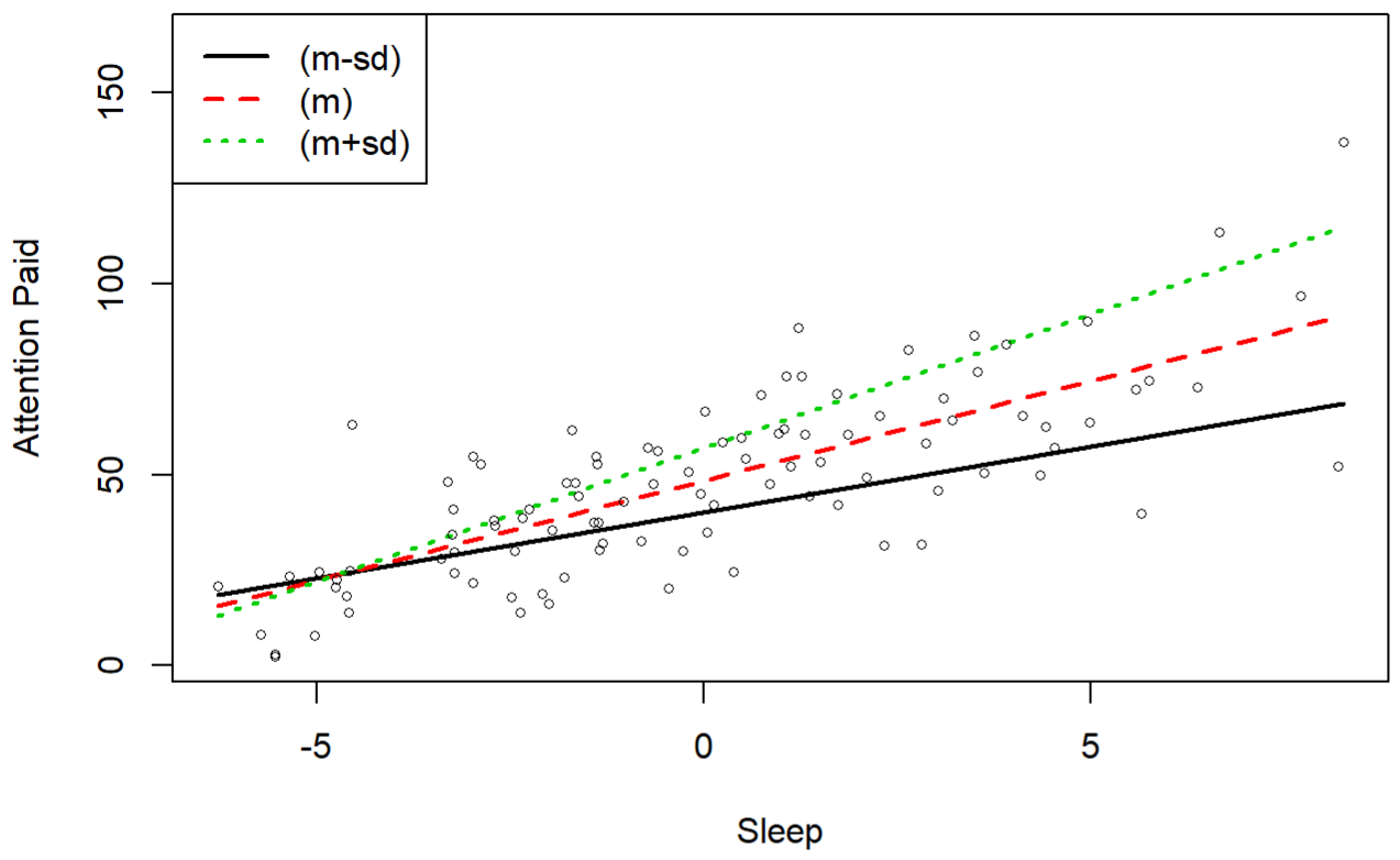
Example: What is the relationship between the number of hours of sleep (X, independent variable (IV)) a graduate student receives and the attention that they pay to this tutorial (Y, outcome) and is this relationship influenced by their consumption of coffee (Z, moderator)
mod <- lm(Y ~ Xc + Zc + Xc*Zc) summary(mod) ## Coefficients: ## Estimate Std. Error t value Pr(>|t|) ## (Intercept) 48.54443 1.17286 41.390 < 2e-16 *** ## Xc 5.20812 0.34870 14.936 < 2e-16 *** ## Zc 1.10443 0.15537 7.108 2.08e-10 *** ## Xc:Zc 0.23384 0.04134 5.656 1.59e-07 ***- Since we have significant interactions in this model, there is no need to interpret the separate main effects of either our IV or our moderator
- Plot the simple slopes (1 SD above and 1 SD below the mean) of the moderating effect
- For details on this plot and analysis, see Regression, Interactions >> OLS >> numeric:numeric >> Calculate simple slopes for the IV at 3 representative values for the moderator variable
- Interpretation
- Those who drank less coffee (moderator, black line) paid more attention (outcome) with the more sleep (IV) that they got last night but paid less attention overall than average (the red line).
- Those who drank more coffee (moderator, green line) paid more attention (outcome) when they slept more (IV) as well and paid more attention than average.
- The difference in the slopes for those who drank more or less coffee (moderator) shows that coffee consumption moderates the relationship between hours of sleep and attention paid
Unobserved Confounds
- Misc
- Packages
- {BiTSLS} - Implements bidirectional two-stage least squares (Bi-TSLS) estimation for identifying bidirectional causal effects between two variables in the presence of unmeasured confounding.
- {causens} - Perform Causal Sensitivity Analyses Using Various Statistical Methods
- {confoundvis} - Provides visualization tools for sensitivity analysis to unmeasured confounding in observational studies.
- Includes contour-based sensitivity plots, robustness curves, and benchmark-oriented graphics that help researchers assess how strong omitted confounding would need to be to attenuate, invalidate, or reverse estimated effects.
- {tipr} - Tools for tipping point sensitivity analyses
- {konfound} (vignette): Utilizes a sensitivity analysis approach that extends from dichotomous outcomes and omitted variable sensitivity of previous approaches to continuous outcomes and evaluates both changes in estimates and standard errors.
- ITCV (Impact Threshold of a Confounding Variable) - Generates statements about the correlation of an omitted, confounding variable with both a predictor of interest and the outcome. The ITCV index can be calculated for any linear model.
- RIR (Robustness of an Inference to Replacement) - Assesses how replacing a certain percentage of cases with counterfactuals of zero treatment effect could nullify an inference. The RIR index is more general than the ITCV index.
- {ovbsa} - Sensitivity Analysis of Omitted Variable Bias
- An observed regressor (or a group of observed regressors) is chosen to benchmark the relative strength of association of the omitted regressor with the outcome variable and with the treatment variable.
- By allowing these sensitivity parameters to take all permissible values, the most conservative estimate of the probability that omitted variable bias can overturn the reported results.
- {senseweight} - Provides tools to conduct interpretable sensitivity analyses for weighted estimators (e.g. survey data)
- Papers
- Hidden yet quantifiable: A lower bound for confounding strength using randomized trials (code)
- Using RCT results and Observational data, this paper proposes a statistical test and a method for determining the lower bound confounder strength.
- In the context of pharmacuticals, RCT results are evidently often released after FDA approval, but this method can be used in any field where there’s a combination of RCT and observational studies.
- When Is Causal Inference Possible? A Statistical Test for Unmeasured Confounding
- This test also uses RCT results and Observational data.
- Hidden yet quantifiable: A lower bound for confounding strength using randomized trials (code)
- Packages
- Handling unobserved confounds is typically done via Partial Identification
- Sometimes the confounding paths of a DAG model can be not be resolved.
- For confounders that influence the treatment and outcome, see:
- Structural Causal Models >> Bayesian examples
- If there’s a mediator, see Other Articles >> Frontdoor Adjustment
- Measure proxies for the unobserved confound if it’s not practical/ethical to measure
- i.e. If the confound is ability, then test scores, letters of recommendation, etc. could be proxies.
- Example: 2022 SR Lecture 10 video, code
.png)
- A: Admitted to Grad School, G: Gender, D: Dept, u: Ability, T1,2,3: 3 Test Scores
- Ability is latent variable/unobserved confounder
- Test Scores are proxies for Ability
- Both models are fit simultaneously
- Couldn’t find a way to use {brms} to code this and Kurz didn’t included it in his brms SR book.
- A: Admitted to Grad School, G: Gender, D: Dept, u: Ability, T1,2,3: 3 Test Scores
- Example: 2022 SR Lecture 10 video, code
- i.e. If the confound is ability, then test scores, letters of recommendation, etc. could be proxies.
- A biased estimate is better than no estimate. It can provide an upper bound
- Find a natural experiment or design one
- Sensitivity Analysis
- After the analyis, you should be able to make the statement, “In order for the confound to be responsible for the entire causal effect, it was have to be this <strength>”
- For confounders that influence the treatment and outcome, see:
- Steps for using sensitivity analysis
- Perform a sensitivity analysis to determine plausibly how much of the causal effect is due to confounding paths
- Assume the confound exists, model it’s consequences for different strengths/kinds of influence
- Example: 2022 SR Lecture 10 video, code
.png)
- A: Admitted to Grad School, G: Gender, D: Dept, u: Unobserved Confounder
- Both models are fit simultaneously
- Values for β and γ are specified and u is estimated as a parameter
- I think Gender (G) is an interaction in both models which I didn’t think was possible given there are no arrows of influence from gender to u.
- Since gender is a moderator it wouldn’t necessarily have to be an influence arrow, it would only need to be an arrow from G to the effect of u on D (see Moderator Analysis), so maybe this is kosher
- Could also be that I’m misunderstanding McElreath’s code he uses to specify his models with {Rethinking}.
- Couldn’t find a way to use {brms} to code this and Kurz didn’t included it in his brms SR book.
- Use previous studies that have effect strengths of those potential confounding variables
- Compare the strengths from the previous studies to the strength determined from the sensitivity analysis. The difference is a good guess for the strength of the causal effect of your treatment variable.
- Perform a sensitivity analysis to determine plausibly how much of the causal effect is due to confounding paths
Statistical Rethinking
Misc
- Arrows indicate directions of influence
- Arrows in DAGs “create” correlations
- i.e. if arrow, then correlation
- The direction it points determines whether its association is causal or not.
- Unlike a statistical model, a DAG, if it is correct, will tell you the consequences of intervening to change a variable.
- ** The data alone can never tell us when a DAG is right. But the data can tell us when a DAG is wrong. **
- Many dynamical systems cannot be usefully represented by DAGs, because they have complex behavior that is sensitive to initial conditions. But these models can still be analyzed and causal interventions designed from them.
- A DAG path means any series of variables you could walk through to get from one variable to another, ignoring the directions of the arrows.
- The variable, U, in DAGs represents one or more unobserved variables
- Usually has circle around the U or is just represented by a dashed line
- “Conditioned upon,” “adjusted for,” or “controlled for” is all the same thing
- “a” or “α” is used in bayesian formulas to represent the intercept
- Notation
- X is not independent of Y, i.e

- conditional independence: Y is not associated with some variable X, after conditioning on some other variable Z, i.e.
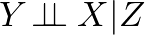
- they are statements of which variables should be associated with one another (or not) in the data.
- they are statements of which variables become dis-associated when we condition on some other set of variables.
- There is no other path of influence from X to Y except through Z
- X is not independent of Y, i.e
- (Total ) Causal Effect and Direct Causal Effect
.png)
- Weight (W) is the outcome, Height (H) and Sex (S) are explanatory
- (Total) Causal Effect is simply, W ~ S
- Direct Causal Effect shuts the backdoor paths, W ~ S + H
- Sometimes we want the total causal effect and not the direct causal effect. (e.g. if H is a post-treatment variable, see SR, Ch.6)
Testable Implications
- Differing associations between plausible DAGs that are testable through statistical models
- Any DAG may imply that some variables are independent of others under certain conditions.
- NO conditional independencies → NO testable implications
- www.dagitty.net - Enter DAG and it will give you the Adjustment Set and Testable Implications
- Example
- Question: What is the causal relationship between Divorce Rate (D), Marriage Rate (M), and Median Age at Marriage (A)
- Data:
- 2 regressions are fit
- D ~ α + βM
- Shows that M is positively correlated with D
- D ~ α + βA
- Shows that A is negatively correlated with D
- D ~ α + βM
- 2 regressions are fit
- Plausible DAGs (note: marriage cannot influence your age… technically)
.png)
- A directly influences D
- M directly influences D
- A directly influences M
- Reasoning: First, Age can have a direct effect, perhaps because younger people change faster than older people and are therefore more likely to grow incompatible with a partner. Second, it can have an indirect effect by influencing the marriage rate. If people get married earlier, then the marriage rate may rise, because there are more young people. Consider for example if an evil dictator forced everyone to marry at age 65. Since a smaller fraction of the population lives to 65 than to 25, forcing delayed marriage will also reduce the marriage rate. If marriage rate itself has any direct effect on divorce, maybe by making marriage more or less normative, then some of that direct effect could be the indirect effect of age at marriage.
.png)
- Similar to 1 except M does not directly influence D
- Reasoning This DAG is plausible even though there’s a correlation between M and D (regression 1). It could be that M derives it’s correlation with D through it’s association with A.
- The direction of influence doesn’t prevent a correlation between M and D
- Testable implications
- DAG 1
- The DAG shows all three are associated to each other, i.e.

- It would be natural to think about measuring correlation and if a pair shows no correlation you could discard the DAG, but it is NOT a good test since there are many ways two variables can show correlation yet not be directly associated. (see reasoning under DAG 2 above and under DAG2 below)
- DAG1 has NO conditional independencies and therefore, NO testable implications
- The DAG shows all three are associated to each other, i.e.
- DAG 2
- This DAG also shows all three variables are associated with each other.
- D and M are associated with one another, because A influences them both. They share a cause, and this leads them to be correlated with one another through that cause. But suppose we condition on A. All of the information in M that is relevant to predicting D is in A. So once we’ve conditioned on A, M tells us nothing more about D
- The testable implication is that D is independent of M, conditional on A, i.e.
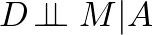
- (Conditioning on A does not make D independent of M, because M really influences D all by itself in this model.)
- i.e A and M are marginally dependent
- (Conditioning on A does not make D independent of M, because M really influences D all by itself in this model.)
- Only difference between both DAGs is the conditional independence in DAG2.
- DAG 1
- Test
- Run a multiple regression D ~ α + βMM + βAA
- If the effect measured from regression 1 disappears in the multiple regression, then we can discard DAG 1. If the effect remains, then we discard DAG 2.
- DAGs that are consistent with the data associations (M & N are associated but the causal relationship isn’t known)
.png)
where U is an unknown variable. Unobserved variables are circled.- All three DAGs have no conditional independencies and therefore not testable implications
- A set of DAGs, each with the same conditional independencies known as a Markov Equivalence
- Data cannot eliminate any of these DAGS. Domain knowledge must be used to reduce the number of Markov Equivalent DAGs.
- All three DAGs have no conditional independencies and therefore not testable implications
“Shutting the backdoor” to potential confounding paths
- Section 6.4
- www.dagitty.net - Enter DAG and it will give you the Adjustment Set and Testable Implications
- Recipe
- List all of the paths connecting X (the potential cause of interest) and Y (the outcome).
- Classify each path by whether it is open or closed. A path is open unless it contains a collider.
- Classify each path by whether it is a backdoor path. A backdoor path has an arrow entering X.
- If there are any backdoor paths that are also open, decide which variable(s) to condition on to close it.
- If you have a choice between two variables where conditioning on either will close a backdoor path and one of them is causal to the outcome variable, then condition on the variable that is causal to the outcome variable. It will add precision to the estimate of the treatment effect.
- Any frontdoor paths that lead to backdoor paths must also be closed (see Misc >> Table 2 fallacy)
- Examples:
.png)
- Problem: We want to measure the causal effect of X –> Y
- Potential confounding paths: XUAC, XUBC
- XUAC doesn’t have a collider so a variable needs conditioned on (aka adjusted for)
- U is unobserved, so either A or C. C directly influences Y, so it’s more efficient and will “aid in precision.”
- XUBC has a collider, B. So, no need to condition on any variable
- XUAC doesn’t have a collider so a variable needs conditioned on (aka adjusted for)
- Solution: Y ~ a + X + C
library(dagitty) dag_6.1 <- dagitty( "dag { U [unobserved] X -> Y X <- U <- A -> C -> Y U -> B <- C }") adjustmentSets( dag_6.1 , exposure="X" , outcome="Y" ) #> { C } #> { A }.png)
- Problem: We want to measure the causal effect of the number of Waffle Houses, W, on Divorce, D.
- Potential confounding paths: WSM, WSA, WSMA (Also WSAM but McElreath on says there are 3. Maybe a combo of same letters is equivalent?)
- WSM doesn’t have a collider and therefore either S or M needs conditioned on
- WSA doesn’t have a collider and therefor either S or A needs conditioned on
- WSMA has a collider, M. So that path is blocked
- M is a choice for WSM but it’s a collider so it’s out. S is in both WSM and WSA, so conditioning on it kills two birds.
- Solution: D ~ a + W + S
library(dagitty)
dag_6.2 <- dagitty( "dag {
    A -> D
    A -> M -> D
    A <- S -> M
    S -> W -> D
}")
adjustmentSets( dag_6.2 , exposure="W" , outcome="D" )
#> { A, M }
#> { S }
Evidently conditioning on A and M is also a solution
- Conditioning on M does close WSM but would then open WSMA. So, by then conditioning on A which is on a fork (or pipe depending on the path) it closes WSMA.
In his brms ebook, Kurz fits these regressions and a couple others for comparison. There wasn’t a consensus point estimate for W in the regressions that adjust for S and A + M.
- McElreath mentions, “This DAG is obviously not satisfactory–it assumes there are no unobserved confounds, which is very unlikely for this sort of data.”
- The inconsistent point estimates are probably do to an omitted variable(s) that is confounding the regression.
Conditional independencies:
impliedConditionalIndependencies( dag_6.2 )
#> A _||_ W | S
#> D _||_ S | A, M, W
#> M _||_ W | S
Other Articles
- Frontdoor Adjustment
- From http://arelbundock.com/posts/frontdoor/
- Useful when an unobserved confounder creates a backdoor path that prevents direct causal estimation
- In a causal chain with three nodes X→Z→Y, we can estimate the effect of X on Y indirectly by combining two distinct quantities:
- The estimate of the effect of X on Z, P(Z|do(X))
- The estimate of the effect of Z on Y, P(Y|do(Z), X)
- Assumptions
- Full mediation: there is no direct path from X to Y, except through Z.
- Un-confoundedness 1: There is no open backdoor from X to Z.
- Un-confoundedness 2: All backdoors from Z to Y are blocked by X
- Example: 1
Our goal is to estimate P(Y|do(X)). Unfortunately, this relationship between X and Y is confounded by the unobserved variable U, via this backdoor path: X←U→Y. Therefore, we cannot estimate the causal quantity of interest directly.
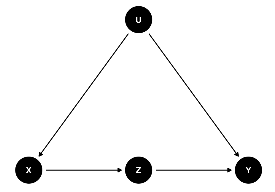
- cause X, a mediator Z, an outcome Y, and an unobserved confounder U
library(data.table)
set.seed(731460)
N = 1e5
U = rbinom(N, 1, prob = .2)
X = rbinom(N, 1, prob = .1 + U * .6)
Z = rbinom(N, 1, prob = .3 + X * .5)
Y = rbinom(N, 1, prob = .1 + U * .3 + Z * .5)
dat = data.table(X, Z, Y)

# truth
coef(lm(Y ~ X + U))["X"]
## 0.2549541
Estimate the effect of X on Z, P(Z|do(X))
step1 = lm(Z ~ X, dat)Estimate the effect of Z on Y, P(Y|do(Z), X)
step2 = lm(Y ~ Z + X, dat)Combine both estimates by multiplication
coef(step1)["X"] * coef(step2)["Z"]
## 0.2496002
- Example 2
Same as first example but using {dosearch} package
library('dosearch') data1 <- "P(X, Y, Z)" query1 <- "P(Y | do(X))" graph1 <- "U -> X U -> Y X -> Z Z -> Y " # compute frontdoor <- dosearch(data1, query1, graph1) frontdoor- Output:
.png)
- Output:
Estimate the causal effect
dat[, `P(X)`    := fifelse(X == 1, mean(X), 1 - mean(X)) ][
    , `P(Z|X)`  := mean(Z), by = X                      ][
    , `P(Y|Z,X)` := mean(Y), by = .(Z, X)                ][
    , `P(Z|X)`  := mean(Z), by = X                      ][
    , Y := NULL                                          ]
dat = unique(dat)
dat[, `P(Y|do(Z))` := sum(`P(Y|Z,X)` * `P(X)`), by = Z]
`P(Y|do(X=0))` = with(dat[X == 0],
  `P(Z|X)`          [Z == 1] *
  `P(Y|do(Z))`      [Z == 1] +
  (1 - `P(Z|X)`)    [Z == 0] *
  `P(Y|do(Z))`      [Z == 0]
)
`P(Y|do(X=1))` = with(dat[X == 1], {
  `P(Z|X)`          [Z == 1] *
  `P(Y|do(Z))`      [Z == 1] +
  (1 - `P(Z|X)`)    [Z == 0] *
  `P(Y|do(Z))`      [Z == 0]
})
`P(Y|do(X=1))` - `P(Y|do(X=0))`
## 0.249766
Comparison
- Truth: 0.2549541
- lm: 0.2496002
- dosearch: 0.249766