Regression
Misc
- Packages
- {kvr2} - Provides functions to calculate nine types of coefficients of determination
- Helps you choose a valid R2 metric for your linear model depending on whether it doesn’t have an intercept, is log-log, or has outliers
- {performance} - Utilities for computing indices of model quality and goodness of fit.
- Metrics such as R-squared (R2), root mean squared error (RMSE), intraclass correlation coefficient (ICC), etc.
- Checks for overdispersion, zero-inflation, convergence, or singularity.
- {olsrr} - Various functions for residuals, heteroskedacity, GOF, etc.
- {kvr2} - Provides functions to calculate nine types of coefficients of determination
Terms
- Collinearity - Umbrella term encompassing any linear association between variables.
- Hat Matrix (AKA Projection Matrix or Influence Matrix) - The matrix that maps the data, \(y\), to the model predictions, \(\hat y\) (i.e. puts “hats” on the predictions). In \(y = A \hat y\), \(A\) is the hat matrix. (source)
- Multicollinearity - Specific type of collinearity where the linear relationship is particularly strong and involves multiple variables.
GOF
{performance}
- Handles all kinds of models including mixed models, bayesian models, econometric models
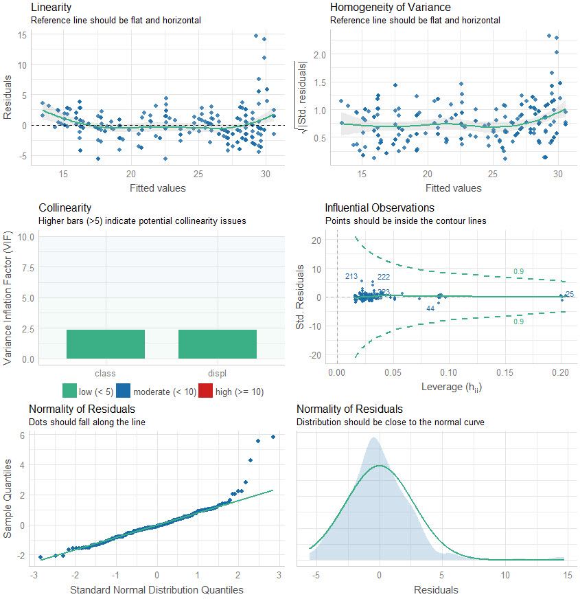
performance::check_model
- Can take a tidymodel as input.
performance::model_performance- Scores model using AIC, AICc, BIC, R2, R2adj, RMSE, Sigma
- “Sigma” is the standard deviation of the residuals (aka Residual standard error, see below)
- Scores model using AIC, AICc, BIC, R2, R2adj, RMSE, Sigma
performance::compare_performance- Outputs table with scores for each model
summary
See Matrix Algebra for Educational Scientists Ch. 29.5 and Ch. 29.6 for details on how these values are calculated
Standard Errors: An estimate of how much estimates would ‘bounce around’ from sample to sample, if we were to repeat this process over and over and over again.
- More specifically, it is an estimate of the standard deviation of the sampling distribution of the estimate.
t-score: Ratio of parameter estimate and its SE
- Used for hypothesis testing, specifically to test whether the parameter estimate is ‘significantly’ different from 0.
p-value: The probability of finding an estimated value that is as far or further from 0, if the null hypothesis were true.
- Note that if the null hypothesis is not true, it is not clear that this value is telling us anything meaningful at all.
F-statistic: This “simultaneous” test checks to see if the model as a whole predicts the response variable better than that of the intercept only (a.k.a. mean) model.
- i.e. Whether or not all the coefficient estimates should jointly be considered unable to be differentiated from 0
- Assumes homoskedastic variance
- If this statistic’s p-value < 0.05, then this suggests that at least some of the parameter estimates are not equal to 0
- Many authors recommend ignoring the P values for individual regression coefficients if the overall F ratio is not statistically significant. This is because of the multiple testing problem. In other words, your p-value and f-value should both be statistically significant in order to correctly interpret the results.
- Unless you only have an intercept model, you have multiple tests (e.g. variables + intercept p-values). There is no protection from the problem of multiple comparisons without this.
- Bear in mind that because p-values are random variables–whether something is significant would vary from experiment to experiment, if the experiment were re-run–it is possible for these to be inconsistent with each other.
Residual standard error - Variation around the regression line.
\[\text{Residual Standard Error} = \sqrt{\frac{\sum_{i=1}^n (Y_i-\hat Y_i)^2}{dof}}\]
- \(\text{dof} = n − k^*\) is the model’s degrees of freedom
- \(k^*\) = The numbers of parameters you’re estimating including the intercept
- Aside from model comparison, can also be compared to the sd of the observed outcome variable
- \(\text{dof} = n − k^*\) is the model’s degrees of freedom
Kolmogorov–Smirnov test (KS)
- Guessing this can be used for GOF to compare predictions to observed
- Misc
- See Distributions >> Tests for more details
- Vectors may need to be standardized (e.g. normality test) first unless comparing two samples
- Packages
- {KSgeneral} has tests to use for contiuous, mixed, and discrete distributions; written in C++
- {stats} and {dgof} also have functions,
ks.test - All functions take a numeric vector and a base R density function (e.g.
pnorm,pexp, etc.) as args - {KSgeneral} docs don’t say you can supply your own comparison sample (2nd arg) only the density function but with stats and dgof, you can.
- Although they have function to compute the CDFs, so if you need speed, it might be possible to use their functions and do it man
g-index
- From Harrell’s rms (doc)
- Note: Harrell often recommends using Gini’s mean difference as a robust substitute for the s.d.
- For Gini’s mean difference, see Feature Engineering, General >> Continuous >> Transformations >> Standardization
- I think the g-index for a model is the total of all the partial g-indexes
- Each independent variable would have a partial g-index
- He also supplies 3 different ways of combining the partial indexes I think
- Harrell has a pretty thorough example in the function doc that might shed light
- Partial g-Index
- Example: A regression model having independent variables,
age + sex + age*sex, with corresponding regression coefficients \(\beta_1\), \(\beta_2\), \(\beta_3\)- g-indexage = Gini’s mean difference (age * (\(\beta_1\) + \(\beta_3\)*w))
- Where w is an indicator set to one for observations with sex not equal to the reference value.
- When there are nonlinear terms associated with a predictor, these terms will also be combined.
- g-indexage = Gini’s mean difference (age * (\(\beta_1\) + \(\beta_3\)*w))
- Example: A regression model having independent variables,
Information Criteria
AIC vs BIC (paper)
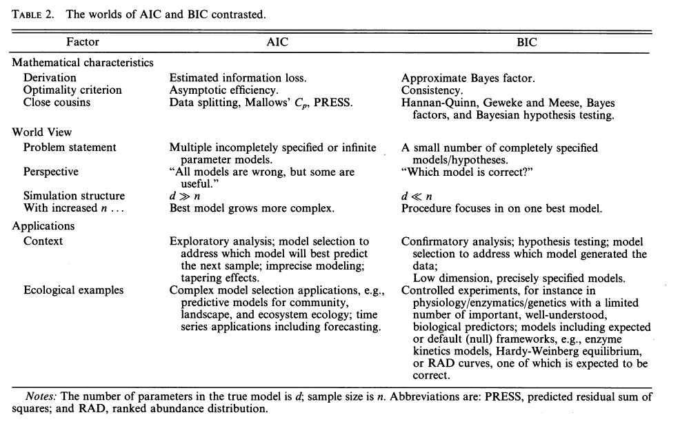
- Lower is Better (which is the model that minimizes the information loss)
- e.g. -754.21 is better than -544.32
- Lower is Better (which is the model that minimizes the information loss)
Assumptions
- Likelihoods of the models being compared is calculated the same way
- e.g. ARIMA and ETS models can’t be compared with AIC or BIC
- The number of observations that the models were trained on must be the same
- A model that uses more lags of a variable than another model will be fit with a different number of observations.
- Likelihoods of the models being compared is calculated the same way
AIC
\[\begin{align} \text{AIC} &= 2k - 2\ln (\hat L) \\ &= T\log \left(\frac{\text{SSE}}{T}\right) + 2(K+2) \end{align}\]
- \(\hat L\) is the maximized likelihood
- \(T\) is the number of observations and \(K\) is the number of parameters
- Penalizes parameters by 2 points per parameter
- Ideal AIC scenario
- Numerous hypotheses are considered
- You have a conviction that all of them are to differing degrees wrong
AICc
\[\text{AIC}_c = \text{AIC} + \frac{2(K+2)(K+3)}{T-K-3}\]
- Small sample size corrected
BIC
\[\text{BIC} = T\log \left(\frac{\text{SSE}}{T}\right) + (K+2)\log(T)\]
- Penalizes parameters by ln(sample size) points per parameter and ln(20) = 2.996
- Almost always a stronger penalty in practice
- Ideal BIC scenario
- Only a few potential hypotheses are considered
- One of the hypotheses is (essentially) correct
Residuals
Misc
- Packages
- {asympDiag} - Generates an envelope plot that compares observed residuals to those expected under the model, helping to identify potential model misspecifications
- {gglm} - Diagnostic plots for residuals
- {infotest} - Information Matrix Test for Regression Models
- Decomposes the test into components for heteroscedasticity, skewness, and kurtosis to diagnose specific forms of misspecification
- {nullabor} (article) - Generates a Null distribution from your residuals. Samples from that distribution to produce a panel of nulll diagnostics plots for comparison against your diagnostic plot. (See example below)
- If your residual plot is indistinguishable from the panel of plots generated by the Null distribution, then there’s no evidence of whichever lack-of-fit issue you’re trying to diagnose.
- If the residual plot is distinguishable, then there is a lack-of-fit issue
- {skedastic} - Implements numerous methods for testing for, modelling, and correcting for heteroskedasticity in the classical linear regression model
influence.measures(mod)wll calculate DFBETAS for each model variable, DFFITS, covariance ratios, Cook’s distances and the diagonal elements of the hat matrix. Cases which are influential with respect to any of these measures are marked with an asterisk.- Cook’s Distance: Different opinions regarding what cut-off values to use. One standard threshold is 4/N (where N = number of observations), meaning that observations with Cook’s Distance > 4/N are deemed as influential
- Scenario: Check of model fit reveals heavy tailed residuals. (Thread)
- The residuals are pretty symmetric, but not just a few outliers.
- Therefore, the concern is mis-estimating standard errors more than mis-estimating the coefficient. (i.e. a violation of the normality of residuals)
- Potential Solutions:
- Use a heavy-tailed error distribution in your original model - Fit the same regression but assume t-distributed errors instead of normal errors. This directly addresses the standard error problem.
- {brms}, {glmmTMB} have a Student-t distribution family
- {mgcv} with family = “scat” for a scaled Student-t distribution
- The location and scale parameter are estimated along with the dof.
- Bootstrap standard errors - Use bootstrap resampling to get empirically-based standard errors that don’t rely on distributional assumptions.
- Sandwich/robust standard errors - These provide consistent standard error estimates even under misspecified error distributions.
- Use a heavy-tailed error distribution in your original model - Fit the same regression but assume t-distributed errors instead of normal errors. This directly addresses the standard error problem.
- Packages
Standardized Residuals:
\[R_i = \frac{r_i}{SD(r)}\]
- Where r is the residuals
- Normalize the residuals to have unit variance using an overall measure of the error variance
- Follows a Chi-Square distribution
- Any \(|R|\) > 2 or 3 is an indication that the point may be an outlier
- In R:
rstandard(mod)rstandard(mod, type = "predictive")provides leave-one-out cross validation residuals, and the “PRESS” statistic (PREdictive Sum of Squares) which issum(rstandard(model, type="pred")^2)
- It may be a good idea to run the regression twice — with and without the outliers to see how much they have an effect on the results.
- Inflation of the MSE due to outliers will affect the width of CIs and PIs but not predicted values, hypothesis test results, or effect point estimates
Studentized Residuals
\[t_i = r_i \left(\frac{n-k-2}{n-k-1-r_i^2}\right)^{\frac{1}{2}}\]
- Where \(r_i\) is the ith standardized residual, \(n\) = the number of observations, and \(k\) = the number of predictors.
- Normalize the residuals to have unit variance using an leave-one-out measure of the error variance
- Some outliers won’t be flagged as outlierrs because they drag the regression line towards them. These residuals are for detecting them.
- Therefore, generally better at detecting outliers than standardized residuals.
- The studentized residuals, \(t\), follow a student t distribution with dof = n–k–2
- Rule of thumb is any \(|t_i|\) > 3 is considered an outlier but you can check the residual against the critical value to be sure.
- In R,
rstudent(mod) - It may be a good idea to run the regression twice — with and without the outliers to see how much they have an effect on the results.
- Inflation of the MSE due to outliers will affect the width of CIs and PIs but not predicted values, hypothesis test results, or effect point estimates
- A Q-Q plot shows the quantiles of the studentized residuals versus fitted values
Check for Normality
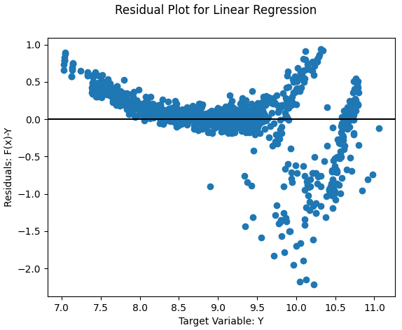
- Residuals vs Fitted scatter
- Looking for data to centered around 0
- Helpful to have a horizontal and vertical line at the zero markers on the X & Y axis.
- Residuals historgram
- Look for symmetry
- Helpful to have a gaussian overlay
- Residuals vs Fitted scatter
Check for heteroskedacity or Other Patterns
- Heteroskedastic
- Breusch Pagan test (
lmtest::bptestorcar::ncvtest)- H0: No heteroskedacity present
bptesttakes data + formula or lm model;ncvtestonly takes a lm model
- Goldfeld-Quandt test (
lmtest::gqtest)- Removes some number of observations located in the center of the dataset, then tests to see if the spread of residuals is different from the resulting two datasets that are on either side of the central observations.
- Must set the fraction of observations to remove — 20% is typical (source)
- e.g. for n = 32, 32*0.20 = 6.4, so around 7. Then set [fraction = 7]{.,arg-text} in
gqtest
- e.g. for n = 32, 32*0.20 = 6.4, so around 7. Then set [fraction = 7]{.,arg-text} in
- H0: Homoskedastic
- Ha: Heteroskedastic
- Megaphone
.png)
- Reverse Megaphone (subtler)
.png)
- Solutions:
- Log transformations of a predictior, outcome or both
- Heteroskedastic robust standard errors (See Econometrics, General >> Standard Errors)
- {modernBoot::wild_boot_lm} - Performs wild bootstrap resampling for linear regression models to handle heteroscedasticity. Supports Rademacher and Mammen weight schemes
- Generalized Least Squares (see Regression, Other >> Misc)
- Weighted Least Squares (see Regression, Other >> Weighted Least Squares)
- Also see Feasible Generalized Least Squares (FGLS) in the same note
- Example: Real Estate >> Appraisal Methods >> CMA >> Market Price >> Case-Shiller method
- {snreg} - Regression with Skew-Normally Distributed Error Term
- Estimate regression models with skew‑normal error terms, allowing both the variance and skewness parameters to be heteroskedastic.
- Includes a stochastic frontier framework that accommodates both i.i.d. and heteroskedastic inefficiency terms.
- Scale model (
greybox::sm) models the variance of the residuals orgreybox::almwill callsmand fit a model with estimated residual variance- See article for an example
- Can be used with other distributions besides gaussian
- The unknown factor or function to describe the residual variance is a problem w/WLS
- {gamlss} also models location, scale, and shape
- Also can be used with other distributions besides gaussian
- Breusch Pagan test (
- Nonlinear
- Solution: Fit a nonlinear model or add a nonlinear transformation to variables
- Example:
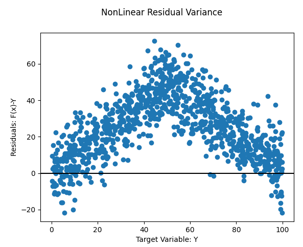
- If you’re unsure about whether you see a pattern or not, try {nullabor}
Example 1: (source)

library(nullabor)

set.seed(1234)

penguins <- penguins |> drop_na(sex)

# remove gentoo species and fit model
ata_no_gentoo <- penguins |>
  filter(species != "Gentoo") |>
  mutate(species = fct_drop(species))

model_no_gentoo <- lm(
  body_mass ~ bill_len + flipper_len + species,
  data = data_no_gentoo
)

fitted_sans_gentoo <- predictions(
  model_no_gentoo,
  newdata = data_no_gentoo
) |>
  mutate(residual = body_mass - estimate)

shuffled_residuals <- lineup(
  null_lm(body_mass ~ bill_len + flipper_len + species, method = "rotate"),
  true = fitted_sans_gentoo,
  n = 9
)

ggplot(shuffled_residuals, aes(x = .fitted, y = .resid)) +
  geom_point() +
  facet_wrap(vars(.sample))

decrypt("sD0f gCdC En JP2EdEPn ZZ")
## Warning in decrypt("sD0f gCdC En JP2EdEPn ZZ"): NAs introduced by coercion
## [1] "nszK w6o6 Xp S4PXoX4p  NA"
If you can’t tell which plot is the original residual plot, then it is unlikely there is a pattern present.
decrypttells us which plot is the original residual plot
Example 2: {nullafor} Non-linearity (source)
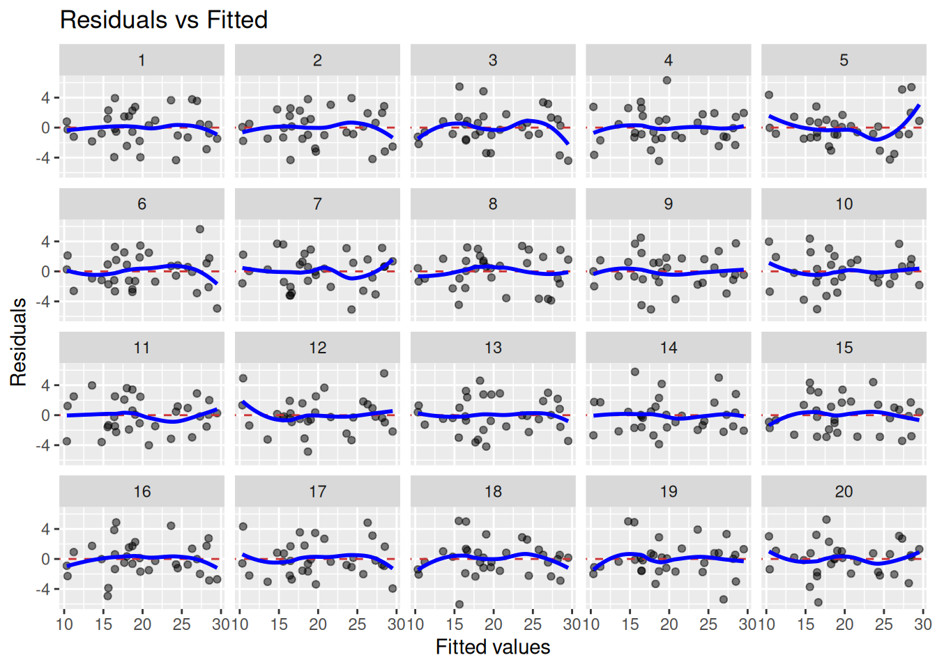
library(nullabor); library(ggplot) mtcars$cyl <- factor(mtcars$cyl) m <- lm(mpg ~ hp + wt + cyl, data = mtcars) m_data <- data.frame(Fitted = predict(m), Residuals = residuals(m)) lineup_residuals(m, type = 1) #> decrypt("Pime gvGv DY FbKDGDbY UR") decrypt("Pime gvGv DY FbKDGDbY UR") #> [1] "True data in position 5"- type = 1 says create residuals vs fitted plots
- 2 = normal Q-Q, 3 = scale-location, 4 = residuals vs leverage
- Styling (color, opacity) also possible within the function, but since it’s a ggplot, I’m sure a theme could be applied.
- Plot 5 sort of sticks out with its slant and extremely whippy tail.
- Other plots have whippy tails and some waviness but not like plot 5
decryptshows us that plot 5 is our plot. This provides evidence of nonlinearity.
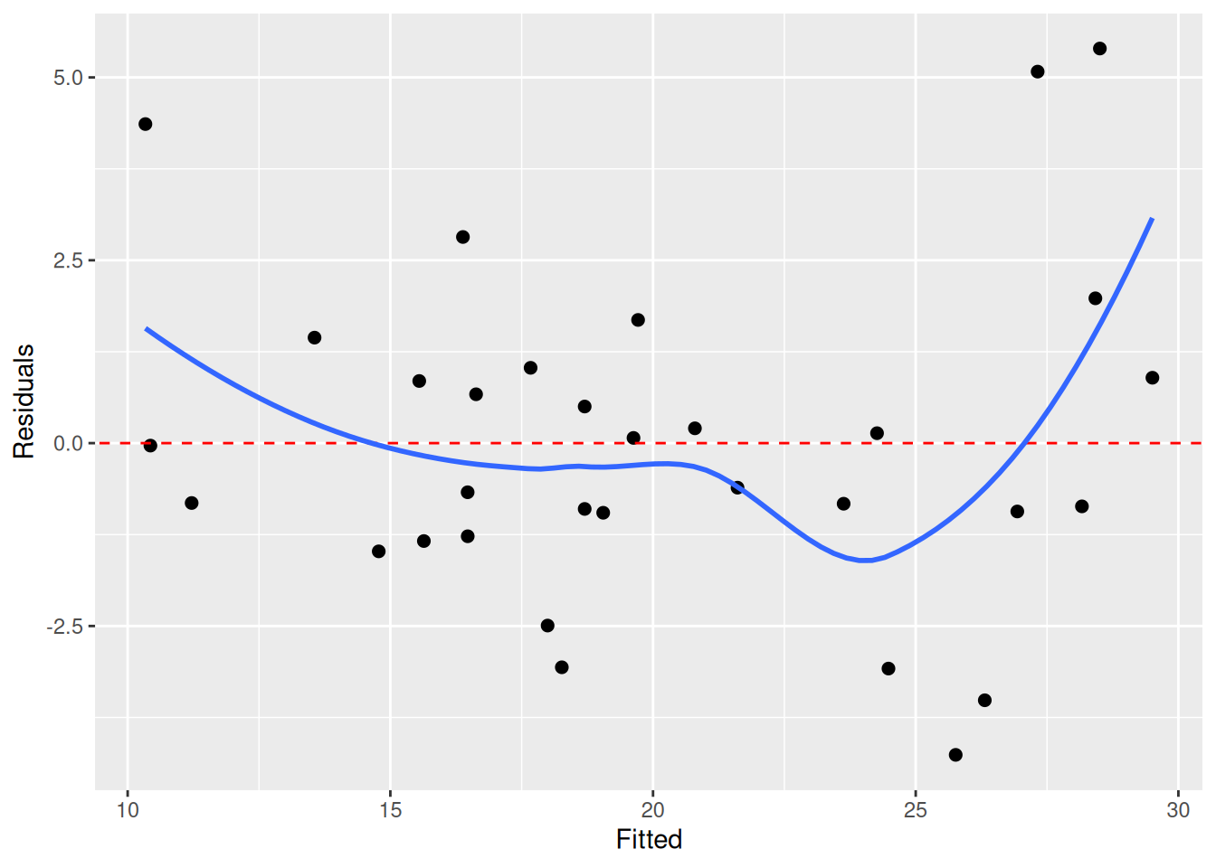
ggplot(m_data, aes(Fitted, Residuals)) + geom_point(size = 2) + geom_abline(aes(intercept = 0, slope = 0), colour = "red", linetype = "dashed") + geom_smooth(se = FALSE)- Now that we have evidence of non-linearity, we can take a closer look at the shape to figure out our next steps (e.g. transformation)
- type = 1 says create residuals vs fitted plots
- Clustering
Example: (source)
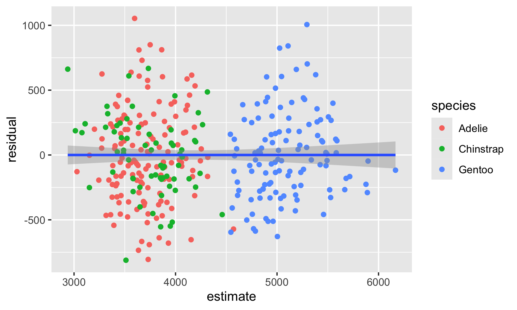
library(tidyverse)       # For ggplot, dplyr, and friends
library(parameters)      # Extract model parameters to data frames
library(marginaleffects)  # Easier model predictions

penguins <- penguins |> drop_na(sex)

model1 <- lm(
  body_mass ~ bill_len + flipper_len + species,
  data = penguins
)

fitted_data <- predictions(model1, newdata = penguins) |>
  mutate(residual = body_mass - estimate)

ggplot(fitted_data, aes(x = estimate, y = residual)) +
  geom_point(aes(color = species)) +
  geom_smooth(method = "lm")
Solutions:
Clustered Standard Errors (See Econometrics, General >> Standard Errors >> Clustered Standard Errors)
Example: Stata-style (source)
parameters::model_parameters(
  model1,
  vcov = "vcovCL",
  vcov_args = list(type = "HC1", cluster = ~species)
)
## Parameter           | Coefficient |     SE |               95% CI | t(328) |      p
## -----------------------------------------------------------------------------------
## (Intercept)         |    -3864.07 | 775.96 | [-5390.56, -2337.58] |  -4.98 | < .001
## bill len            |       60.12 |  12.75 | [   35.03,    85.20] |   4.71 | < .001
## flipper len         |       27.54 |   4.69 | [   18.32,    36.77] |   5.87 | < .001
## species [Chinstrap] |     -732.42 | 116.67 | [ -961.92,  -502.91] |  -6.28 | < .001
## species [Gentoo]    |      113.25 | 120.60 | [ -123.99,   350.50] |   0.94 | 0.348
##
## Uncertainty intervals (equal-tailed) and p-values (two-tailed) computed using a Wald t-distribution approximation.
- Heteroskedastic
Check for Autocorrelation
- Run Durbin-Watson, Breusch-Godfrey tests:
forecast::checkresiduals(fit)to look for autocorrelation between residuals.- Range: 1.5 to 2.5
- Close to 2 which means you’re in the clear.
- Run Durbin-Watson, Breusch-Godfrey tests:
Check for potential variable transformations
- Residual vs Predictor
- Run every predictor in the model and every predictor that wasn’t used.
- Should look random.
- Nonlinear patterns suggest non linear model should be used that variable (square, splines, gam, etc.). Linear patterns in predictors that weren’t use suggest they should be used.
car::residualPlots- Plots predictors vs residuals and performs curvature test- p < 0.05 –> Curvature present and need a quadratic version of the variable
- Or
car::crPlots(model)for just the partial residual plots
- {ggeffects}
- Introduction: Adding Partial Residuals to Marginal Effects Plots
- Shows how to detect not-so obvious non-linear relationships and potential interactions through visualizing partial residuals
- Introduction: Adding Partial Residuals to Marginal Effects Plots
- Harrell’s {rms}
- Logistic regression example (link)
- End of section 10.5; listen to audio
- Logistic regression example (link)
- Residual vs Predictor
plot(fit)
- For each fitted model object look at residual plots searching for non-linearity, heteroskedacity, normality, and outliers.
- The correlation matrix (see bkmk in stats) for correlation and VIF score (See below) for collinearity among predictors.
- Also see Regression, Linear >> Linear Algebra for the correlation matrix and link to code
- Collinearity/Multicollinearity Issues:
- Model can’t distinguish the individual effects of each predictor on the response variable. It captures the shared variance with other correlated predictors. Consequently, small changes in the data can lead to significant fluctuations in the estimated coefficients, potentially leading to misleading interpretations.
- Inflation of the variance of the coefficient estimates results in wider confidence intervals which makes it harder to detect significant effects.
- If non-linearity is present in a variable run poly function to determine which polynomial produces the least cv error
- Is heteroscedasticity is present use a square root or log transform on the variable. Not sure if this is valid with multiple regression. If one variable is transformed the others might have to also be transformed in order to maintain interpretability. *try sandwich estimator in regtools, car, or sandwich pkgs*
- Outliers can be investigated further with domain knowledge or other statistical methods
- Example: Diamonds dataset from {ggplot2}
price ~ carat + cut
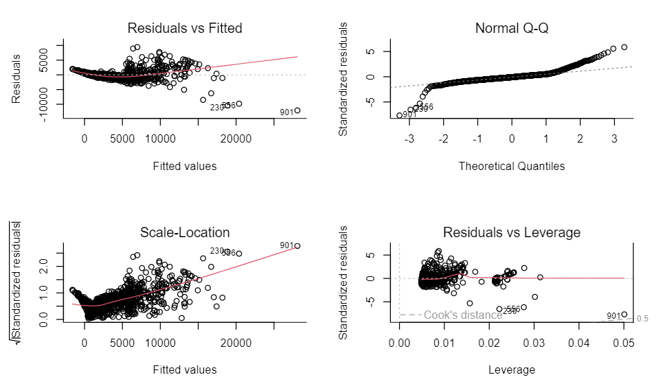
- Bad fit
- Residuals vs Fitted: Clear structure in the residuals, not white noise. They curve up at the left (so some non-linearity going on), plus they fan out to the right (heteroskedasticity)
- Scale-Location: The absolute scale of the residuals definitely increases as the expected value increases — a definite indicator of heteroskedasticity
- Normal Q-Q: Strongly indicates the residuals aren’t normal, but has fat tails (e.g. when they theoretically would be about 3 on the standardised scale, they are about 5 - much higher)
log(price) ~ log(carat) + cut
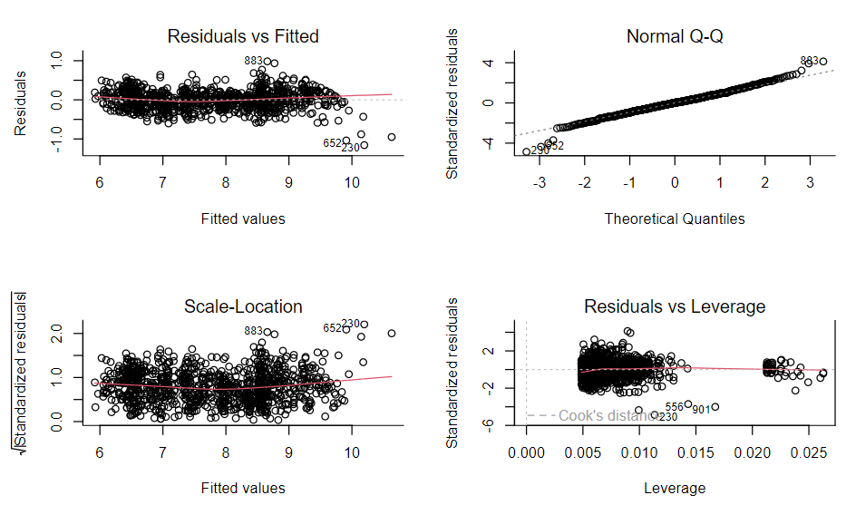
- Good fit
- Residuals vs Fitted: Curved shape and the fanning has gone and we’re left with something looking much more like white noise
- Scale-Location: Looks like solid homoskedasticity
- Normal Q-Q: A lot more “normal” (i.e. straight line) and apart from a few outliers the values of the standardized residuals are what you’d expect them to be for a normal distribution
Other Diagnostics
Misc
- Tutorial for modeling with Harrell’s {Hmisc}
- {kernelshap} and {fastshap} can handle complex lms, glms (article)
- Also see Diagnostics, Model Agnostic >> SHAP
Check for influential observations - outliers that are in the extreme x-direction
Check VIF score for collinearity (source)
- If prediction is the goal, multicollinearity probably isn’t a problem
- Although if future values of the collinear predictor are outside the range of the training data, then predictions become unreliable (at least in forecasting) (source)
- Options for interpretting coefficients:
- Interpret coefficients jointly rather than individually
- Acknowledging the uncertainty in individual coefficient estimates
- Consider whether your research question truly requires separating the effects of correlated predictors
- For interaction terms, high VIF values are expected and often unavoidable. This is sometimes called “inessential ill-conditioning.” Centering the component variables can sometimes help reduce VIF values for interactions
- Sometimes, multicollinearity reflects important aspects of your data or research question. Removing variables to reduce VIF may actually harm your analysis by omitting important confounders or by changing the interpretation of remaining coefficients
- If prediction is the goal, multicollinearity probably isn’t a problem
For prediction, if coefficients vary significantly across the test folds their robustness is not guaranteed (see coefficient boxplot below), and they should probably be interpreted with caution.
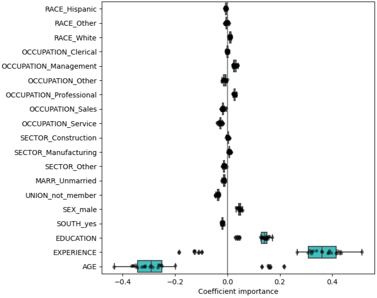
- Boxplots show the variance of the coefficient across the folds of a repeated 5-fold cv.
- The “Coefficient importance” in the example is just the coefficient value of the standardized variable in a ridge regression
- Note outliers beyond the whiskers for Age and Experience
- In this case, the variance is caused by the fact that experience and age are strongly collinear.
- Variability in coefficients can also be explained by collinearity between predictors
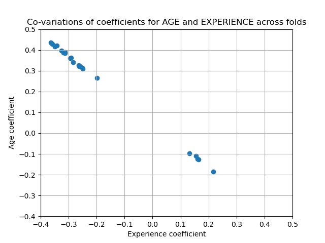
- Perform sensitivity analysis by removing one of the collinear predictors and re-running the CV. Check if the variance of the variable that was kept has stabilized (e.g. fewer outliers past the whiskers of a boxplot).
step_lincomb- Finds exact linear combinations between two or more variables and recommends which column(s) should be removed to resolve the issue. These linear combinations can create multicollinearity in your model.example_data <- tibble( a = c(1, 2, 3, 4), b = c(6, 5, 4, 3), c = c(7, 7, 7, 7) ) recipe(~ ., data = example_data) |> step_lincomb(all_numeric_predictors()) |> prep() |> bake(new_data = NULL) # A tibble: 4 × 2 a b <dbl> <dbl> 1 1 6 2 2 5 3 3 4 4 4 3
ML Prediction
Misc
Get test predictions from tidymodels workflow fit obj
preds_tbl <- wflw_fit_obj %>%
    predict(testing(splits)) %>%
    bind_cols(testing(splits), .)
Calibration
- {tailor} - Postprocessing of predictions for tidymodels;
Creates an object class for performing calibration that can be set used with workflow objects, tuning, etc. Diagnostics of calibration seems to remain in {probably}.
For numeric outcomes: calibration, truncate prediction range
Truncating ranges involves limiting the output of a model to a specific range of values, typically to avoid extreme or unrealistic predictions. This technique can help improve the practical applicability of a model’s outputs by constraining them within reasonable bounds based on domain knowledge or physical limitations.
See introduction to the package for a calibration example
Correlated Errors 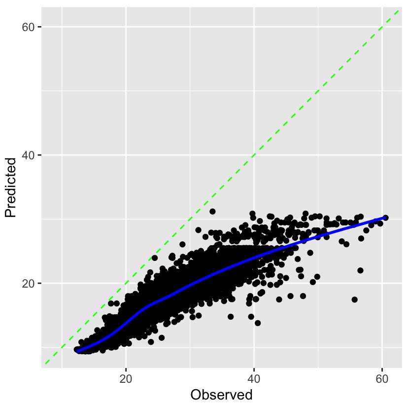
Calibrated Predictions 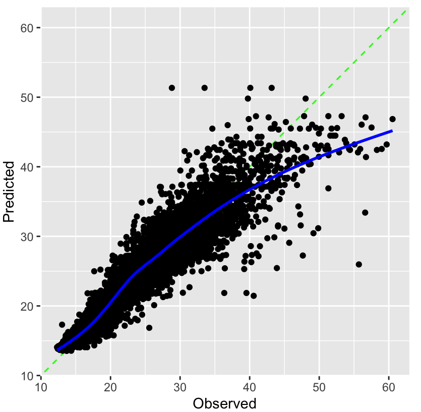
- {tailor} - Postprocessing of predictions for tidymodels;
GOF
RMSE/sd(target variable) Ratio
Guidelines
Ratio (RMSE/SD) Interpretation < 0.50 Good predictive ability 0.50 – 0.70 Moderate predictive ability 0.70 – 0.90 Weak predictive ability > 0.90 Model barely beats the mean RMSE penalizes outliers very harshly (quadratic), so your residuals need to be fairly normaly and symmetric.
The SD is also a poor summary of spread for skewed distributions.
Alternatives
- Heavy tails / outliers → MAE / MAD ratio
- Not the same guidelines as RMSE / sd but they rhyme:
- A ratio near 1.0 means your model barely beats the naive baseline
- A ratio well below 0.5 suggests strong predictive ability
- Not the same guidelines as RMSE / sd but they rhyme:
- Heavy tails → RMSE on log-transformed target or use RMSLE
- Note that errors on the log scale correspond to relative (multiplicative) errors on the original scale, so you’re implicitly changing what “error” means.
- RMSLE (root mean squared log error) is essentially RMSE applied after a \(\log(1+y)\) transform.
- Heavy tails / outliers → MAE / MAD ratio
RMSE of model vs naive
RMSE penalizes outliers very harshly (quadratic), so your residuals should be fairly normal (no long or fat tails).
Code
preds_tbl %>%
    yardstick::rmse(outcome_var, .pred)
preds_tbl %>%
    mutate(.naive = mean(outcome_var)) %>%
    yardstick::rmse(outcome_var, .naive)
R2
preds_tbl %>% yardstick::rsq(outcome_var, .pred)- Squared correlation between truth and estimate to guarantee a value between 0 and 1
Observed vs Predicted plot
preds_tbl %>%
    ggplot(aes(outcome_var, .pred)) +
    # geom_jitter(alpha = 0.5, size = 5, width = 0.1, height = 0) + # if your outcome var is discrete
    geom_smooth()
Feature Importance
Example: tidymodel xgboost
xgb_feature_imp_tbl <- workflow_obj_xgb %>%
    extract_fit_parsnip() %>%
    pluck("fit") %>%
    xgboost::xgb.importance(model = .) %>%
    as_tibble() %>%
    slice(1:20)

xgb_feature_imp_tbl %>%
    ggplot(aes(Gain, fct_rev(as_factor(Feature)))) %>%
    geom_point()