Other
Misc
- Packages
- {brtobit}
- Estimation and inference from generalized linear models using various methods for bias reduction
- Can be used in models with Separation (See Diagnostics, GLM >> Separation)
- Reduction of estimation bias is achieved by solving either:
- The mean-bias reducing adjusted score equations in Firth (1993) and Kosmidis & Firth (2009)
- The median-bias reducing adjusted score equations in Kenne et al (2017)
- The direct subtraction of an estimate of the bias of the maximum likelihood estimator from the maximum likelihood estimates as prescribed in Cordeiro and McCullagh (1991).
- {bsamGP} (Vignette) - Bayesian Spectral Analysis Models using Gaussian Process Priors
- Currently the package includes parametric linear models, partial linear additive models with/without shape restrictions, generalized linear additive models with/without shape restrictions, and density estimation model.
- Provides a Bayesian method for shape-restricted regressions with monotone, convex/concave, S-shaped and U-shaped curves
- MCMC sampling written in Fortran90
- The prior for the unknown function is based on an infinite series expansion with a Karhunen-Loève representation of a second-order Gaussian process.
- Currently the package includes parametric linear models, partial linear additive models with/without shape restrictions, generalized linear additive models with/without shape restrictions, and density estimation model.
- {fastfrechet} (JOSS) - A fast, scalable, and user-friendly implementation of both Fréchet regression and variable selection for 2-Wasserstein space
- The squared Euclidean norm in linear regression is replaced by a general distance function which depends on the type of response.
- Response type examples
- A probability distribution (e.g., a density or cumulative distribution function)
- e.g. a mortality distribution for country, i, in year, ti, where t is a predictor
- Wasserstein distance
- A correlation matrix
- e.g. a correlation matrix summarizing connectivity between brain regions for subject, i, with age as a predictor
- Frobenius distance
- A shape, image, or function
- e.g. modeling how average MRI brain scans (as a 3D function or 2D slice) change with age (Voxel-wise L2 or Structural similarity (SSIM))
- e.g. how the shape of a leaf (2D boundary curve or set of landmarks) changes depending on environmental variables (Procrustes distance or elastic shape distance (via square-root velocity functions))
- e.g. a person’s growth curve (height measurements over a time interval) from their birth weight (L2)
- A point on a manifold (like the sphere, S2)
- e.g. Modeling animal movement direction (unit vector) based on temperature (Geodesic)
- A probability distribution (e.g., a density or cumulative distribution function)
- {kernreg} - Fast implementation of Nadaraya-Watson kernel regression for either univariate or multivariate responses, with one or more bandwidths. K-fold cross-validation is also performed.
- {outrigger} (Paper) - Performs outrigger regression
- A nonparametric regression function, called an outrigger estimator, that is designed to adapt to the unknown error distribution (which may in particular be non-Gaussian)
- {brtobit}
- Papers
- Paper: An interpretable family of projected normal distributions and a related copula model for Bayesian analysis of hypertoroidal data (angular data)
- Example: In meteorology
- Examples of angular data include wave directions in environmental science, directions of animal movement in biology, dihedral angles in protein backbone structures in bioinformatics, and times of crimes in political science.
- Paper: An interpretable family of projected normal distributions and a related copula model for Bayesian analysis of hypertoroidal data (angular data)
- Harrell: It is not appropriate to compute a mean or run parametric regression on “% change” unless you first compute
log((%_change/100) + 1)to undo damage done by % change - Reaction time data can be modelled using several families of skewed distributions (Lindeløv, 2019)
Other
- Rates between 0 and 1
- Also see Confidence and Prediction Intervals >> Conformal Prediction Intervals >> Misc >> Papers for conformal intervals for bounded 0-1 data models
- Outcome without 0s and 1s
- Beta Regression
- {gkwreg} - Implements regression models for bounded continuous data in the open interval (0,1) using the five-parameter Generalized Kumaraswamy distribution
- {SelectBoost.beta} - Stability-Selection via Correlated Resampling for Beta-Regression Models
- {ZeroOneDists} - Zero-one statistical distributions for estimating parameters and fitting regression models within the GAMLSS framework
- Outcome with 0s and 1s
- Extended support Beta Regression (Zeileis), aka XBX Regression
- {betaregscale} - An alternative to {betareg}
- Provides a mixed-effects extension via multivariate Laplace approximation for repeated measures and multi-centre data.
- betareg issues:
- Interpretability: It relies on a mean-precision parameterization (μ,ϕ) where the precision parameter ϕ lacks a direct, clinically intuitive meaning.
- Measurement Resolution: It ignores the discretized nature of rating scales. Selecting “52” on an NRS-101 reflects a measurement interval [0.515,0.525], not a precise continuous value. Ignoring this leads to underestimated residual variance and biased inference.
- betaregscale solutions:
- Mean-Dispersion (MD) Parameterization: Reparameterizes the beta distribution in terms of the conditional mean μ∈(0,1) and a proportional dispersion parameter σ∈(0,1), both directly interpretable and modelable via covariates.
- Interval-Censored Likelihood: Properly treats each discrete scale point as interval-censored data, integrating the beta PDF over the uncertainty bounds implied by the instrument’s resolution. A score of y* on a K-point scale is treated as \(y^*_{K - 1}/(2K): y^*_{K + 1}/(2K)\)
- Ordered Beta Regression
- Zero-inflated or Zero-1-inflated beta regression (ZOIB) (see {brms})
- If the zeros and ones are censored, use tobit.
- Quasi-Binomial GLM
Uses the logit link from logistic regression, but allows the relationship between the mean and variance to be larger (or smaller) by some consistent ratio.
- Note that a binomial response forces the variance to equal to \(p(1-p)/n\), not just be proportional to it.
Example: GLM (source)
model2 <- glm(per_gop ~ cpe, family = quasibinomial, data = combined, weights = total_votes) summary(model2) #> Coefficients: #> Estimate Std. Error t value Pr(>|t|) #> (Intercept) -1.82178 0.06823 -26.70 <2e-16 *** #> cpe 9.25748 0.34153 27.11 <2e-16 ***- per_gop: Percentage of votes cast for the Republican presidential candidate
- cpe: Crude Prevalence Estimate; depression measure
- Counties weighted based on their overall number of voters, which makes particular sense for a binomial or similar family response.
Example: Mixed Effects GAM (source)
# must be a factor to use as a random effect in gam(): combined <- mutate(combined, state_name = as.factor(state_name)) model5 <- gam(per_gop ~ cpe + s(state_name, bs = 're'), family = quasibinomial, weights = total_votes, data = combined) #> Parametric coefficients: #> Estimate Std. Error t value Pr(>|t|) #> (Intercept) -3.2466 0.2802 -11.59 <2e-16 *** #> cpe 16.3333 0.6224 26.24 <2e-16 *** #> --- #> Signif. codes: 0 ‘***’ 0.001 ‘**’ 0.01 ‘*’ 0.05 ‘.’ 0.1 ‘ ’ 1 #> #> Approximate significance of smooth terms: #> edf Ref.df F p-value #> s(state_name) 48.44 49 20.54 <2e-16 ***- Varying intercepts model
- Lets the vote for Trump in any state vary for all the state-specific things that aren’t in our model
- Doing so, let’s us see if we still get an overall (constant nation-wide) relationship between depression and voting in the counties within each state.
{betaboost} - Boost beta regression via mboost and gamboostLSS. Repo is old so not sure if it’s still viable. Follows {betareg} API
{cobin} (Paper) - Cobin and micobin regression models
- Cobin and micobin regression models are scalable and robust alternative to beta regression model for continuous proportional data.
- Outcome variable is greater than 0
- Gamma Regression - Can handle some dispersion with a log link
- Can model multiplicative dgp
- If zero-inflated, use Tweedie Regression
- Bounded Outcome Variable
- Tweedie Regression - Where the frequency of events follows a Poisson distrbution and the amount associated with each event follows an Exponential distribution
- Generalized Least Squares
- Packages
- {nlme::gls}
- Math - A Deep-Dive into Generalized Least Squares Estimation
- Also See Weighted Least Squares and Weighted Least Squares >> Feasible Generalized Least Squares
- Packages
- One-Inflated
- Packages
- {oneinfl} - Estimates one-inflated positive Poisson (OIPP) and one-inflated zero-truncated negative binomial (OIZTNB) regression models.
- Packages
Censored and Truncated Data
Packages
- {FMCensSkewReg} - Finite Mixture of Censored Regression Models with Skewed Distributions
- Normal (FM-NCR), Student t (FM-TCR), skew-Normal (FM-SNCR), and skew-t (FM-STCR).
- Enables flexible modeling of skewness and heavy tails often observed in real-world data, while explicitly accounting for censoring.
- {ModalCens} - Implements parametric modal regression for continuous positive distributions of the exponential family under right censoring.
- Provides functions to link the conditional mode to a linear predictor using reparameterizations for Gamma, Beta, Weibull, and Inverse Gaussian families
- {FMCensSkewReg} - Finite Mixture of Censored Regression Models with Skewed Distributions
Censored Data - Arise if exact values are only reported in a restricted range. Data may fall outside this range but those data are reported at the range limits (i.e. at the minimum or maximum of the range)
- i.e. Instances outside the range are recorded in the data but the true values of those instances are not.
- It can be done purposely in order to better the model fit. From a paper that models precipitation, “fitting is improved by censoring the data, so in practice we remove values \(Y (x) < 0.5 \text{(mm)}\). Other thresholds (\(\le 0.2\) and \(\le 0.1\text{mm}\)) have been tested but \(Y (x) < 0.5 \text{(mm)}\) gives the best results, in particular for the upper tails.”
- Tobit Regression - regression models with a Gaussian response variable left-censored at zero, assumes constant (homoskedastic variance)
Log-Likelihood function
\[ \ln \mathcal{L}(\beta, \sigma^2) = \sum_{i=1}^N \left[d_i\left(\frac{1}{2}\ln 2\pi - \frac{1}{2}\ln \sigma^2 - \frac{1}{2\sigma^2} (y_i - \boldsymbol{x}_i'\beta)^2\right) + (1-d_i) \ln \left(1-\Phi(\frac{\boldsymbol{x}_i' \beta}{\sigma}\right)\right] \]
- \(d_i = 0\) if \(y_i = 0\), and \(1\) otherwise
- 1st term OLS likelihood
- 2nd term accounts for the probability that observation i is censored.
- \(d_i = 0\) if \(y_i = 0\), and \(1\) otherwise
Marginal Effect
\[ \frac{\partial \mathbb{E}(y|x)}{\partial x} = \beta_1 \left[\Phi \left(\frac{\beta_0 + \beta_1 x}{\sigma}\right) \right] \]- \(\beta_1\) is multiplied by the CDF (\(\Phi\)) of the Normal distribution
- \(\beta_1\) is weighted by the probability of y occurring at \(x\)
- Example: work_completed ~ hourly rate
- \(\beta_1\) is weighted by the probability that an individual is willing to work at the present hourly rate, as represented by the CDF.
- \(\sigma\) is the standard deviation of the model’s residuals
- \(\beta_1\) is multiplied by the CDF (\(\Phi\)) of the Normal distribution
Example: Right-Censored at 800
VGAM::vglm(resp ~ pred1 + pred2,
           family = tobit(Upper = 800),
           data = dat)
- 2-Part Models (e.g. Hurdle Models) - A binary (e.g. Probit) regression model fits the exceedance probability of the lower limit and a truncated regression model fits the value given the lower limit is exceeded.
Truncated Data - Arise if exact values are only reported in a restricted range. If data outside this range are omitted completely, we call it truncated
- i.e. Instances outside the range are NOT recorded. No evidence of these instances are in the data.
- Truncated Regression - Also assumes constant (homoskedastic variance)
- A poisson model will try to predict zeros even if zeros are impossible. Therefore, you need a zero-truncated model.
- The truncated normal model is different from a glm, because \(\mu\) and \(\sigma\) are not orthogonal and have to be estimated simultaneously. Misspecification of one parameter will lead to inconsistent estimation of the other. That’s why for these models, not only is \(\mu\) often specified as a function of regressors but also \(\sigma\), often in the framework of GAMLSS (generalized additive models of location, scale, and shape).
- Expectation: \(E[y|x] = \mu + \sigma + \frac {\phi(\mu / \sigma)}{\Phi(\mu / \sigma)}\)
- Where \(\phi(\cdot)\) and \(\Phi(\cdot)\) are the probability density and cumulative distribution function of the standard normal distribution, respectively. This intrinsically depends on both \(\mu\) and \(\sigma\).
- Expectation: \(E[y|x] = \mu + \sigma + \frac {\phi(\mu / \sigma)}{\Phi(\mu / \sigma)}\)
Heteroskadastic Variance - The variance of an underlying normal distribution does depend on covariates
- {crch}
Examples
- Insurance: There is a claim on a policy that has a payout limit of \(u\) and a deductible of \(d\),
- Any loss amount that is greater than \(u\) will be reported to the insurance company as a loss of \(u - d\) because that is the amount the insurance company has to pay.
- Insurance loss data is left-truncated because the insurance company doesn’t know if there are values below the deductible \(d\) because policyholders won’t make a claim.
- “Truncated” because the values (claims) are below \(d\), so the instances aren’t recorded in the data.
- “Left” because the values are below \(d\) and not above
- Insurance loss data is also right-censored if the loss is greater than \(u\) because \(u\) is the most the insurance company will pay. Thus, it only knows that your claim is greater than \(u\), not the exact claim amount.
- “Censored” because the values (claims) that are exactly \(u\) (policy limit) imply that claim is greater than \(u\), so the instances are recorded but the true values are unknown.
- “Right” because the values are above \(u\) and not below
- Measuring Wind Speed: The instrument needs a minimum wind speed, \(m\), to start working.
- If wind speeds below this minimum are recorded as the minimum value, \(m\), the data is censored.
- i.e. Some other instrument detects a wind instance occurred and that instance is recorded as \(m\) even though the true speed of the wind of that instance is unknown.
- If wind speeds below this minimum are NOT recorded at all, the data is truncated.
- i.e. Any wind instances (detected or not) are not recorded. No evidence in the data that these instances will have ever occurred.
- If wind speeds below this minimum are recorded as the minimum value, \(m\), the data is censored.
- Insurance: There is a claim on a policy that has a payout limit of \(u\) and a deductible of \(d\),
Fractional Regression
- Outcome with values between 0 and 1
- ** Use a fractional logit (aka quasi-binomial) only for big data situations **
- The fractional logit model is not a statistical distribution, leading it to produce biased results.
- See Kubinec article
- Recommends ordered beta regression, continuous bernoulli and provides examples
- In a big data situation, it respects the bounds of proporitional/fractional outcomes, and is significantly easier to fit than the other alternatives.
- Having a large dataset means that inefficiency or an incorrect form for the uncertainty of fractional logit estimates is unlikely to affect decision-making or inference.
- Beta: values lie between zero and one
- See {betareg}, {DirichletReg}, {mgcv}, {brms}
- {ordbetareg}
- Zero/One-Inflated Beta: larger percentage of the observations are at the boundaries (i.e. high amounts of 0s and 1s
- See {brms}, {VGAM}, {gamlss}
- Logistic, Quasi-Binomial, or GAM w/robust std.errors: outcome, y, is \(0 \le y \le 1\) (i.e. 0s and 1s included)
Example
library(lmtest)
library(sandwich)
# logistic w/robust std.errors
model_glm = glm(
  prate ~ mrate + ltotemp + age + sole,
  data = d,
  family = binomial
)
se_glm_robust <- coeftest(model_glm, vcov = vcovHC(model_glm, type="HC"))
# quasi-binomial w/robust std.errors
model_quasi = glm(
  prate ~ mrate + ltotemp + age + sole,
  data = d,
  family = quasibinomial
)
se_glm_robust_quasi = coeftest(model_quasi, vcov = vcovHC(model_quasi, type="HC"))

# Can also use a GAM to get the same results
# Useful for more complicated model specifications
model_gam_re = gam(
  prate ~ mrate + ltotemp + age + sole + s(id, bs = 're'),
  data = d,
  family = binomial,
  method = 'REML'
)
Zero-Inflated and Zero-Truncated
- Also see Regression, Discrete
- Continuous
- Some economists will use \(\ln(1 + Y)\) or \(\mbox{arcsinh}(Y)\) to model a skewed, continous \(Y\) with \(0\)s. In this case, the treatment effects (ATE) can’t be interpreted as percents. The effect sizes will depend on the scale of \(Y\). (see Thread)
- Solutions
Normalize \(Y\) by a pretreatment baseline
\[ Y' = \frac{Y}{Y_{\text{pre}}} \]
- Where \(Y_{\text{pre}}\) is the measured \(Y\) prior to treatment
- In regression, average treatment effect (ATE) would then be
\[ \theta_{\bar Y} = \mathbb{E} \left[\frac{Y(1)}{Y_{\text{pre}}} - \frac{Y(0)}{Y_{\text{pre}}} \right] \]- Where \(Y(1)\) is the value of \(Y\) for treated subjects
- Interpretation (e.g outcome = earnings): average treatment effect on earnings expressed as a percentage of pre-treatment earnings
Normalizing \(Y\) by the expected outcome given observable covariates
\[ Y' = \frac{Y}{\mathbb{E}[Y(0) \:|\: X]} \]
- \(Y(0)\) are the observed outcome values for the control group
- The “\(|X\)” is kind of confusing but I don’t think want the fitted values from a model where the outcome is the \(Y(0)\) values. I think they’d use a \(\hat Y\) somewhere.
- So I think \(\mathbb{E}[Y(0) | X]\) just the mean of the \(Y(0)\) values
- Interpretation of this transformed variable (e.g. outcome = earnings)
- an individual’s earnings as a percentage of the average control group’s earnings for people with the same observable characteristics X.
- Average Treatment Effect (ATE) Interpretation (e.g. outcome = earnings, \(X\) = pretreatment earnings, education)
- The average change in earnings as a percentage of the control group’s earnings for people with the same education and previous earnings.
- ML 2-step Hurdle
- Steps
- Transform Target variable to 0/1 where 1 is any count that isn’t a 0.
- Use a classifier to predict 0s (according to some probability threshold)
- Remember that models is predicting the probability of being a 1
- Filter rows that aren’t predicted to be 0, and predict counts using a regressor model
- round-up or round-down predictions based on which results in lower error?
- Steps
- Statistical
- Options: Poission, Neg.Binomial, Zero-Inf Poisson/Neg.Binomial, Poisson/Neg.Binomial Hurdle
- Zero-Inf Poisson/Neg.Binomial
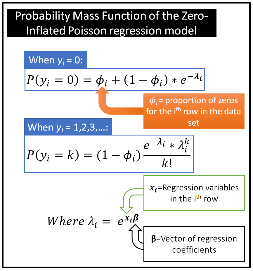
- Uses a second underlying process that determines whether a count is zero or non-zero. Once a count is determined to be non-zero, the regular Poisson process takes over to determine its actual non-zero value based on the Poisson process’s PMF.
- ϕi is the predicted probability from a logistic regression that yi is a 0. This vector of values is then plugged into both probability mass functions.
- Zero-Inflated Weibull
- Packages
- {ZIDW} - Parameter estimation for zero-inflated discrete Weibull (ZIDW) regression models
- Includes distribution functions, functions to generate randomized quantile residuals, a pseudo R2, and plotting of rootograms
- {ZIDW} - Parameter estimation for zero-inflated discrete Weibull (ZIDW) regression models
- Packages
Multi-modal
- Also see EDA, General >> Continuous Variables >> Check Shape of Distribution
- Packages
- {DEmixR} - Fits, bootstraps, and evaluates two-component normal and lognormal mixture models.
- Includes diagnostic plots and statistical evaluation of mixture model fits using differential evolution optimization.
- {DEmixR} - Fits, bootstraps, and evaluates two-component normal and lognormal mixture models.
- Models
- Quantile Regression
- Mixture Model
- Establish cutpoints and model each modal distribution separately
- ML
Weighted Least Squares (WLS)
OLS with Weighted Pbservations
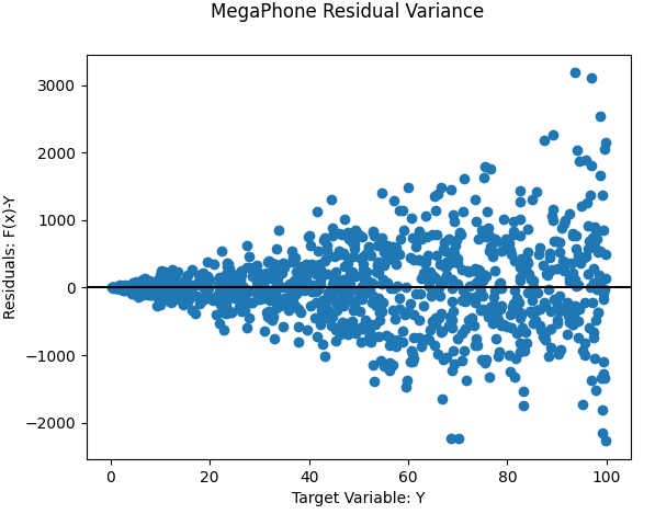
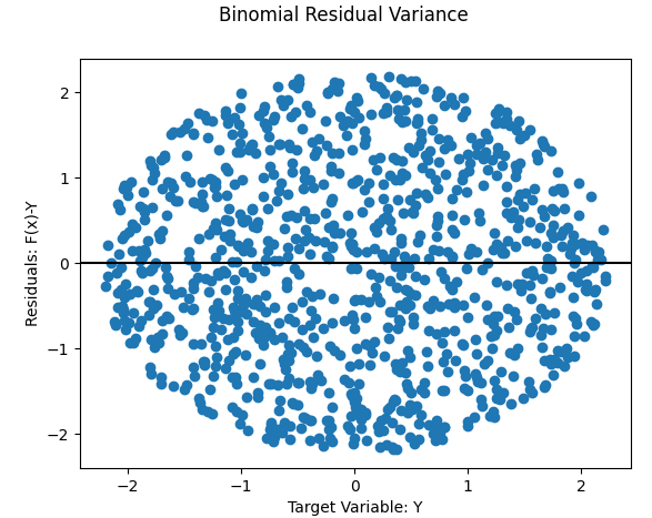
Commonly used to overcome binomial or “megaphone-shaped” types of heteroskedacity of OLS residuals
Misc
- Also see
- Other >> Generalized Least Squares
- Real Estate >> Appraisal Methods >> CMA >> Market Price >> Case-Shiller Method for an example
- Resources
- R >> Documents >> Econometrics >> applied-econometrics-in-r-zeileis-kleiber >> pg 76
- Feasible Generalized Least Squares (FGLS) seems to have advantages over WLS Allows you to find the “form of the skedastic function to use and… estimate it from the data” * See Zeileis applied econometrics book or another econometrics book for details
- Also see
The residual error to be minimized becomes:
\[ \begin{align} J(\hat \beta) &= \mathbb{E} [(f(x) - y)^2]\\ & = \sum_i^n (w_i f(x_i) - y_i)^2\\ & = \sum_i^n (w_ix_i^T \beta - y_i)^2 \end{align} \]- Where \(w_i\) is the weight assigned to observation \(i\)
\(\hat \beta\) becomes \((X^T WX)^{-1}XY\)
- Where \(W\) is a diagonal matrix containing the weights for each observation
For “megaphone-shaped” and binomial types of heteroskedacity, it’s common to set the weights to equal to each observation’s squared residual error
\[ w_i = (f(x_i)-y_i)^2 \]
Generalized Estimating Equations (GEE)
- Models that are used when individual observations are correlated within groups. Often used when repeated measures (panel data) for an individual are collected over time.
- You make a good guess on the within-subject covariance structure. The model averages over all subjects, and instead of assuming that data were generated from a certain distribution, it uses moment assumptions to iteratively choose the best \(\beta\) to describe the relationship between covariates and response.
- Semiparametric Method: Some structure on the data generating process (linearity) is imposed, the distribution is not fully specified. Estimating \(\beta\) is purely an exercise in optimization.
- Limitations
- Likelihood-based methods are not available for usual statistical inference. GEE is a quasi-likelihood method and therefore less flexible.
- Unclear on how to perform model selection, as GEE is just an estimating procedure. There is no goodness-of-fit measure readily available.
- No subject-specific estimates: If that is the goal of your study, use a different method.
- Other Options
- Generalized Linear Mixed Model (GLMM) - GLMMs require some parametric assumptions (See Mixed Effects, GLMM)
- *Note that the interpretations of the resulting estimates are different for GLMM and GEE*
- Generalized Joint Regression Modelling (GJRM)
- Generalized Linear Mixed Model (GLMM) - GLMMs require some parametric assumptions (See Mixed Effects, GLMM)
- Scenarios
- You are a doctor. You want to know how much a statin drug will lower your patient’s odds of getting a heart attack.
- GLMM answers this question
- Sounds like a typical logistic regression parameter interpretation
- You are a state health official. You want to know how the number of people who die of heart attacks would change if everyone in the at-risk population took the statin drug.
- GEE answers this question. GEE estimates population-averaged model parameters and their standard errors
- Sounds like a typical linear regression parameter interpretation
- You are a doctor. You want to know how much a statin drug will lower your patient’s odds of getting a heart attack.
- Misc
- Notes from
- Packages
- {gee}: traditional implementations (only has a manual)
- {geepack}: traditional implementations (1 vignette)
- Can also handle clustered categorical responses
- {multgee}: GEE solver for correlated nominal or ordinal multinomial responses using a local odds ratios parameterization
- {geess} - Modified Generalized Estimating Equations for Small-Sample Data
- The traditional GEE implementation has severe computation challenges and may not be possible when the cluster sizes (large numbers of individuals per cluster) get too large (e.g. >1000)
- Use One-Step Generalized Estimating Equations method (article with code)
- Operates under the assumption of exchangeable correlation (see below)
- Characteristics
- Matches the asymptotic efficiency of the fully iterated GEE;
- Uses a simpler formula to estimate the [intra-cluster correlation] ICC that avoids summing over all pairs;
- Completely avoids matrix multiplications and inversions for computational efficiency
- Use One-Step Generalized Estimating Equations method (article with code)
- Assumptions
- The responses \(Y_1, Y_2, \ldots , Y_n\) are correlated or clustered
- There is a linear relationship between the covariates and a transformation of the response, described by the link function, \(g\).
- Within-cluster covariance has some structure (“working covariance”)
- Individuals in different clusters are uncorrelated
- Covariance Structure
- Need to pick one of these working covariance structures in order to fit the GEE
- Types
- Independence: observations over time are independent
- Exchangeable (aka Compound Symmetry): all observations over time have the same correlation
- Correlation across individuals is constant within a cluster
- Intra-Cluster Correlation (ICC) is the measure of this correlation.
- AR(1): correlation decreases as a power of how many timepoints apart two observations are
- Reasable if measurements taken closer together (i.e. probably more highly correlated)
- Unstructured: correlation between all timepoints may be different)
- If the wrong covariance structure is chosen, β will be estimated consistently, even if the working covariance structure is wrong. However, the standard errors computed from this will be wrong.
- To fix this, use Huber-White “sandwich estimator” (HC standard errors) for robustness. (See Econometrics, General >> Standard Errors)
- The idea behind the sandwich variance estimator is to use the empirical residuals to approximate the underlying covariance.
- Problematic if:
- The number of independent subjects is much smaller than the number of repeated measures
- The design is unbalanced — the number of repeated measures differs across individuals
- To fix this, use Huber-White “sandwich estimator” (HC standard errors) for robustness. (See Econometrics, General >> Standard Errors)
- Example: {geepack}
Description: How does Vitamin E and copper level in the feeds affect the weights of pigs?
Data
library("geepack") data(dietox) dietox$Cu <- as.factor(dietox$Cu) dietox$Evit <- as.factor(dietox$Evit) head(dietox) ## Weight Feed Time Pig Evit Cu Litter ## 1 26.50000 NA 1 4601 1 1 1 ## 2 27.59999 5.200005 2 4601 1 1 1 ## 3 36.50000 17.600000 3 4601 1 1 1 ## 4 40.29999 28.500000 4 4601 1 1 1 ## 5 49.09998 45.200001 5 4601 1 1 1 ## 6 55.39999 56.900002 6 4601 1 1 1- Weight of slaughter pigs measured weekly for 12 weeks
- Starting weight (i.e. the weight at week (Time) 1 and Feed = NA)
- Cumulated Feed Intake (Feed)
- Evit is an indicator of Vitamin E treatment
- Cu is an indicator of Copper treatment
Model: Independence Working Covariance Structure
mf <- formula(Weight ~ Time + Evit + Cu) geeInd <- geeglm(mf, id=Pig, data=dietox, family=gaussian, corstr="ind") summary(geeInd) ## Coefficients: ## Estimate Std.err Wald Pr(>|W|) ## (Intercept) 15.07283 1.42190 112.371 <2e-16 *** ## Time 6.94829 0.07979 7582.549 <2e-16 *** ## Evit2 2.08126 1.84178 1.277 0.258 ## Evit3 -1.11327 1.84830 0.363 0.547 ## Cu2 -0.78865 1.53486 0.264 0.607 ## Cu3 1.77672 1.82134 0.952 0.329 ## --- ## Signif. codes: 0 '***' 0.001 '**' 0.01 '*' 0.05 '.' 0.1 ' ' 1 ## ## Estimated Scale Parameters: ## Estimate Std.err ## (Intercept) 48.28 9.309 ## ## Correlation: Structure = independenceNumber of clusters: 72 Maximum cluster size: 12- corstr=“ind” is the argument for the covariance structure
- See article for examples of the other structures and how they affect estimates
- corstr=“ind” is the argument for the covariance structure
ANOVA
anova(geeInd)

## Analysis of 'Wald statistic' Table
## Model: gaussian, link: identity
## Response: Weight
## Terms added sequentially (first to last)
##
##      Df  X2 P(>|Chi|)
## Time  1 7507    <2e-16 ***
## Evit  2    4      0.15
## Cu    2    2      0.41
## ---
## Signif. codes:  0 '***' 0.001 '**' 0.01 '*' 0.05 '.' 0.1 ' ' 1