Geospatial
Misc
- Also see Real Estate >> Features
- Resources
- Feature Engineering A-Z, Ch. 105
- Safegraph data
- Misc
- $200 free credits
- {SafeGraphR}
- article
- Measure foot traffic
- Locate where you customers come from
- Misc
Latitude and Longitude Transformations
- Also see
- Engineered >> Bin Latitude and Longitude
- Feature Engineering >> Splines >>
- When the area covered by the data is large, the difference between using ellipsoidal coordinates and projected coordinates will automatically become larger and will have an effect on predictive modeling.
- For very large extents and global models, polynomials or splines in latitude and longitude will not work well as they ignore the circular nature of longitude and the coordinate singularities at the poles. Here, spherical harmonics, base functions that are continuous on the sphere with increasing spatial frequencies can replace polynomials or be used as spline base functions. (source)
- Most of these transformations are for geographic coordinate systems (e.g. ESPG: 4326) and not projected coordinate systems (e.g. EPSG: 25832)
For projected coordinate systems, it’s best to scale (e.g. min/max) . Then, create low-level interactions (\(X \times Y\)), quadratics (\(X^2\) , \(Y^2\)), and splines (e.g. thin plate)
Example: (source >> Example 1)
sf_pm10_feat <- sf_pm10 |> sf::st_drop_geometry() |> mutate( X = sf::st_coordinates(sf_pm10)[, 1], Y = sf::st_coordinates(sf_pm10)[, 2], x_scaled = (X - min(X)) / (max(X) - min(X)), y_scaled = (Y - min(Y)) / (max(Y) - min(Y)), ) spline_spec <- mgcv::s(x_scaled, y_scaled, bs = "ts", k = 10) ls_coord_splines <- mgcv::smoothCon( spline_spec, sf_pm10_feat[, c("x_scaled", "y_scaled")] ) mat_splines <- ls_coord_splines[[1]]$X colnames(mat_splines) <- paste0("spline_", 1:10) sf_pm10_feat <- sf_pm10_feat |> bind_cols(as_tibble(mat_splines))- A similar workflow would work for geographical coordinates (i.e. latitude and longitude)
- Decimal to Degrees, Minutes, Secs
- Example: 123.875
- Degrees: 123
- Minutes: .875 \(\times\) 60 = 52.5 \(\rightarrow\) 52 minutes
- Seconds: 0.5 (from minutes calculation) \(\times\) 60 = 30 seconds
- Example: 123.875
- Round
- Round to longitude and latitude to 3 or 4 decimal places
- Radians
- Convert the latitude and longitude to radians
- Geocode
- Geocode Addresses to latitude and longitude
- {tidygeocoder}
Basic
new_tbl <- old_tbl %>%
    geocode(
        address = <address_var>, #e.g. "city, state"
        method = "arcgis"
    )
Multiple Geocoders
tib_coords_prosp <- tib_addrs |> tidygeocoder::geocode_combine( queries = list( list(method = 'census', full_results = TRUE, api_options = list(census_return_type = 'geographies')), list(method = 'osm'), list(method = 'arcgis') ), global_params = list(address = 'addrs_full'), cascade = TRUE ) |> select(1:4, 11:15)- See Scraping >> API >> GET >> Example: Real Estate Addresses for a look at the tib_addrs dataset
- Each method in the queries list is a geocoding API
- For method = ‘census’, full_results = TRUE and census_return_type = ‘geographies’ are both required to get census tracts, FIPS codes, etc.
- global_params passes that argument to all methods
- cascade = TRUE says whichever addresses can’t be geocoded by census, feed (only) those to osm, and whichever addresses don’t get coded by osm get fed to arcgis.
- Reverse Geocode
latitude and longitude to Addresses
Create categoricals like city, state, country
If the coordinates are in the same city, for example, then extracting the street address would be necessary
{tidygeocoder}
new_tbl <- old_tbl %>% reverse_geocode( lat = "<latitude_var>", long = "<longitude_var>", address = "estimated_address", # disired column name for result method = "arcgis" )- Outputs street address, city, state, zip, country
- Cosine and Sine
Cyclical variable (0° - 360°) (e.g. slope aspect)
new_var <- cos(old_var) * pi / 180) new_var <- sin(old_var) * pi / 180)- If there’s a specific azimuth direction (or point in the cycle) where you expect the maximum or minimum, you can shift the aspect variable before calculating the (co)sine.
Latitude and Longitude
x = cos(lat) * cos(lon) y = cos(lat) * sin(lon) z = sin(lat)- Latitude and Longitude are 2-D coordinates representing a 3-D system. This transforms them to 3-D.
- To Decimal
Zip Codes
- Issues
- There are 10K Point ZIP codes out of ~42K US ZIP codes and only ~32K ZIP codes have a physical boundary
- Every country has its own ZIP code system
- Aren’t necessarily a location
- e.g. US Navy, which has its own ZIP code, but no permanent location
- Types - PO Box, Unique (individual addresses), Military, and Standard
- Might be easier to work with Zip Code Tabulation Areas (ZCTAs) (see bkmks Geospatial >> Resources >> Shapefiles)
- See zip_code_database.csv in R >> Data for different attributes of all the US zipcodes (lat, long, cities, population, etc.)
- Hashing might be a good approach (See Feature Engineering, General >> Categorical >> Encoding/Hashing)
Engineered
- Spatial Lags
For each location, the average value of the variable is calculated for a set of neighbor locations.
Each lag is associated with a unique set of neighbors.
As lags increase, the further away the set of neighbors is from origin location
See Geospatial, Spatial Weights >> Diagnostics >> Connectedness for further details
Packages
- {ebtools::add_spatial_lags} - Creates higher order spatial lags
Adding spatially lagged independent variables can make models robust to a range of possible mis-specifications (source)
- Entity boundaries should be arbitrary, or not designed for the data collection process
- Useful especially if spatial processes in the dependent variable and/or the residuals are unclear
Example: First order lag (source)
pacman::p_load(dplyr, sfdep)
data(guerry, package = "sfdep")

lag_crime_per <-
  guerry |>
  transmute(
    nb = st_contiguity(geometry),
    wt = st_weights(nb),
    crime_lag1 = st_lag(crime_per, nb, wt)
  ) |>
  pull(crime_lag1)
- Distance from
- Distance from a school, supermarket, movie theater, interstate, highway, industrial park, etc.
- Distance from the nearest city, Distance to the nearest big city
- The Harvsine Formula takes into account the Earth’s curvature for a more accurate distance
- Nearest Location
- Examples: Nearest city name, Nearest big city, Nearest city population
- Cluster Lat/Long
- Cluster longitude and latitude and then one-hot encode the cluster labels
- DBSCAN and Hierarchical is supposed to work best with geospatial features
- Binning and Crossing
“Crossing” is multiplying 1 boolean column times another or more boolean columns
Binning prevents a change in latitude producing the same result as a change in longitude (?)
You can also bin latitude and longitude to different granularities such as by neighborhood or city block to provide info about those areas
If the column is continuous, then it needs to be binned and one-hot encoded before being crossed
Binning and crossing latitude and longitude with a 3rd binned feature provides area info about that 3rd predictor to the model
- Example binned_latitude x binned_longitude x binned_traffic_stops where latitude and longitude are binned by city block
- Provides the model with info about traffic stops at the city block granularity
- Example binned_latitude x binned_longitude x binned_traffic_stops where latitude and longitude are binned by city block
Pseudo code
binned_latitude(lat) = [ 0 < lat <= 10 10 < lat <= 20 20 < lat <= 30 ] binned_longitude(lon) = [ 0 < lon <= 15 15 < lon <= 30 ] # crossing the binned features binned_latitude_X_longitude(lat, lon) = [ 0 < lat <= 10 AND 0 < lon <= 15 0 < lat <= 10 AND 15 < lon <= 30 10 < lat <= 20 AND 0 < lon <= 15 10 < lat <= 20 AND 15 < lon <= 30 20 < lat <= 30 AND 0 < lon <= 15 20 < lat <= 30 AND 15 < lon <= 30 ]- i.e. both conditions true –> 1, either condition false –> 0
Cyclic var
bin_cycl_var <- function(x) { cut((x + 22.5) %% 360, breaks = seq(0,360,by=45), labels = c("N","NE","E","SE","S","SW","W","NW")) }- Sine/Cosine transform or cyclic smoothing spline will probably produce better results
- Bin Lat/Long Then Transform
- Embed: use categorical embedding
- Might be better to bin, cross, then embed
- Or depending on the number of unique pairs, maybe just cross and embed
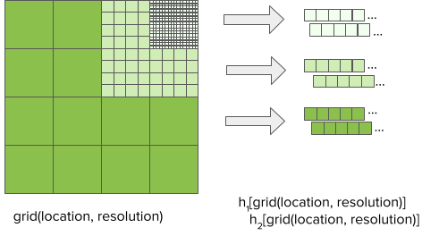
- Exact Indexing: maps each grid cell to a dedicated embedding. This takes up the most space.
- Feature Hashing: maps each grid cell into a compact range of bins using a hash function. The number of bins is much smaller than with exact indexing.
- “While feature hashing saved space compared to exact indexing, the accuracy was the same or slightly worse depending on the grid resolution. This is likely due to hash collisions that cause some information to be lost” (from Uber ETA model article, also see Deep Learning, Tabular >> Architectures >> DeepETA: Uber’s ETA model)
- Multiple Feature Hashing: extends feature hashing by mapping each grid cell to multiple compact ranges of bins using independent hash functions
- “Provided the best accuracy and latency while still saving space compared to exact indexing. This implies that the network is able to combine the information from multiple independent hash buckets to undo the negative effects of single-bucket collisions.” (from Uber ETA model article, also see Deep Learning, Tabular >> Architectures >> DeepETA: Uber’s ETA model)
- I think this means they binned longitude and latitude at 3 different grid resolutions, then each cell is hashed twice with 2 independent hashing functions. This results in 6 features(?)
- Embed: use categorical embedding
- Cyclic Smoothing Spline
- Also see Feature Engineering, Splines >> Misc >> Use Cases for Spline Types
- Paper shows Thin Plate Splines being used for latitude and longitude
mgcv::s(cyclic_var, bs = "cc", k = k)- k lets you optionally control the e.d.f. to avoid overfitting
- Example used k = 10
- k lets you optionally control the e.d.f. to avoid overfitting
- Effective Degrees of Freedom (EDF):
- The effective degrees of freedom (EDF) quantify the complexity of the spline model. It is defined in a way that takes into account the smoothing parameter.
- The EDF can be thought of as the equivalent number of parameters that are effectively used by the spline to fit the data.
- It is given by the trace of the smoothing matrix, which maps the observed data to the fitted values.
- Interpretation:
- A higher EDF indicates a less smooth spline that fits the data more closely (potentially overfitting).
- A lower EDF indicates a smoother spline that may not capture all the nuances of the data (potentially underfitting).
- Also see Feature Engineering, Splines >> Misc >> Use Cases for Spline Types
- kNN x Lags
- Haven’t tried this and it’s surely implemented by someone, but this method seems like the closest analog to the way outcome variable lags are used as predictors in autoregression in order to handle autocorrelation. I’d think this method would help account for spatial autocorrelation
- Calculate centroids. Then for each centroid, find its k nearest neighbors by distance.
Example: Calculate County Centroids
library(dplyr)
library(sf)

# Get 2023 shape files
download.file('https://www2.census.gov/geo/tiger/GENZ2023/shp/cb_2023_us_county_500k.zip',
              destfile = "../../Data/cb_2023_us_county_500k.zip", mode = "wb")

unzip("../../Data/cb_2023_us_county_500k.zip")

counties <- st_read("cb_2023_us_county_500k.shp")
county_cent <- counties |>
  st_centroid()

sc <- st_coordinates(county_cent)

county_cent <- county_cent |>
  mutate(long = sc[, 1],
         lat = sc[, 2],
         # combine the two digit state code with the 3 digit county code to join w/other data
         county_fips = paste0(STATEFP, COUNTYFP))
- For each nearest neighbor, multiply its distance from the centroid of interest by a lag of that neighbor’s outcome value
- If applicable, divide the values by a scaling factor (e.g. population)
- Each nearest neighbor’s final value is a predictor value (e.g. using 5 neighbors will result in 5 predictors)
- Example: Find 5 closest county centroids by distance to Jefferson County’s centroid . Multiply those distances times the lagged COVID cases value of those countries. Lastly divide each of those values by its population
- Tuning parameters: lags and number of nearest neighbors.