Analysis

Misc

Also see
- Domain Knowledge >> Epidemiology >> Disease Mapping

Terms

Areal (aka Lattice) Data - Arise when a study region is partitioned into a limited number of areas, with outcomes being aggregated or summarized within those areas
Buffer - a zone around a geographic feature containing locations that are within a specified distance of that feature, the buffer zone. A buffer is likely the most commonly used tool within the proximity analysis methods. Buffers are usually used to delineate protected zones around features or to show areas of influence.
Catchment - The area inside any given polygon is closer to that polygon’s point than any other. Refers to the area of influence from which a retail location, such as a shopping center, or service, such as a hospital, is likely to draw its customers. (also see Retail >> Catchment)
Spatial Functional Data - Data comprising curves or functions that are recorded at each spatial location.

Proximity Analysis

Example: Basic Workflow
- Data: Labels, Latitude, and Longitude
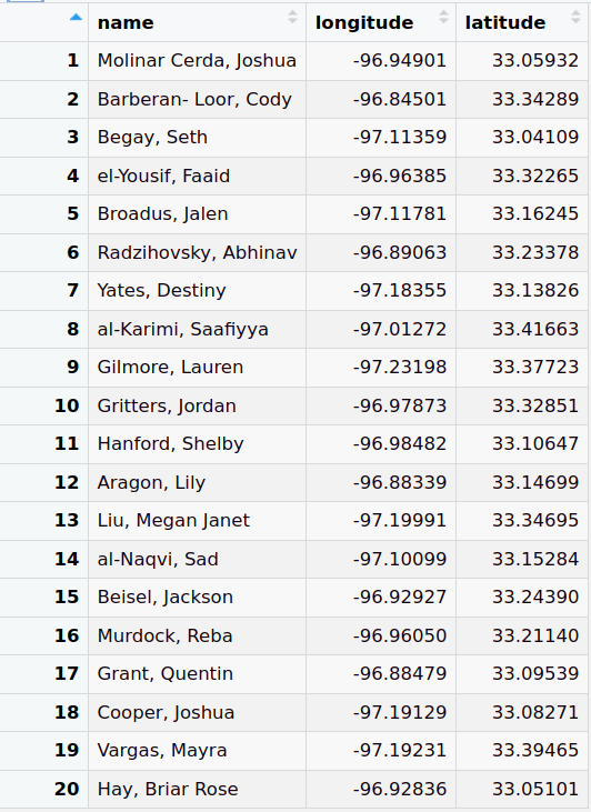
- Create Simple Features (sf) Object
```
customer_sf <- 
  customer_table %>%
    sf::st_as_sf(coords = c("longitude", "latitude"),
                 crs = 4326)
```
  - Merges the longitude and latitude columns into a geometry column and transforms the coordinates in that column according to projection (e.g. crs = 4326)
- View points on a map
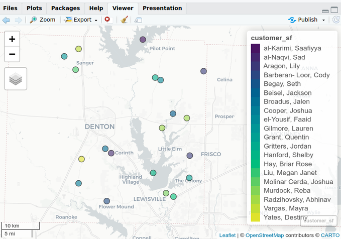
```
mapview::mapview(customer_sf)
```
- Create Buffer Zones
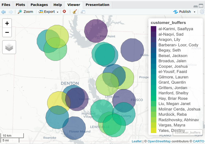
```
customer_buffers <- 
  customer_sf %>%
    sf::st_transform(26914) %>%
    sf::st_buffer(5000)

mapview::mapview(customer_buffers)
```
  - Most of projections use meters, and based on the size of the circles as related to the size of Denton, TX, I’m guessing the radius of each circle is 5000m. Although, that still looks a little small.
- Create Isochrones
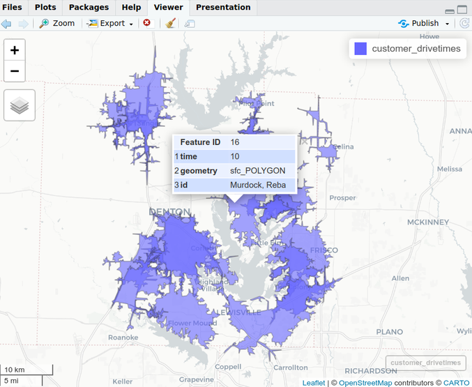
```
customer_drivetimes <- 
  customer_sf %>%
    mapboxapi::mb_isochrone(time = 10, 
                            profile = "driving", 
                            id_column = "name")

mapview::mapview(customer_drivetimes)
```
  - 10 minutes drive-time from each location
  - time (minutes): The maximum time supported is 60 minutes. Reflects traffic conditions for the date and time at which the function is called.
    - If reproducibility of isochrones is required, supply an argument to the depart_at argument.
  - depart_at: Specifying a time makes it a time-aware isochrone. Useful for modeling peak business hours or rush hour traffic, etc.
    - e.g. Adding depart_at = “2024-01-27T17:30” to the isochrone above gives you a 10-minute driving isochrone with predicted traffic at 5:30pm tomorrow
- Add Demographic Data
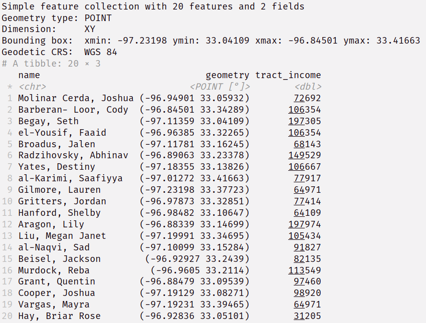
```
denton_income <- 
  tidycensus::get_acs(
    geography = "tract",
    variables = "B19013_001",
    state = "TX",
    county = "Denton",
    geometry = TRUE
  ) %>%
    select(tract_income = estimate) %>%
    sf::st_transform(st_crs(customer_sf))

customers_with_income <- customer_sf %>%
  sf::st_join(denton_income)

customers_with_income
```
  - Adds median income estimate according to the census tract each person lives in.
  - Joins on the geometry variable
Circular Buffer Approach
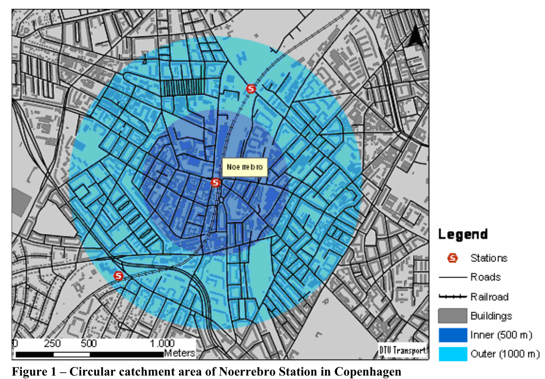
- Notes from GIS-based Approaches to Catchment Area Analyses of Mass Transit
- The simplest and most common used approach to make catchment areas of a location is to consider the Euclidean distance from the location.
- Due to limitations (See below), it’s best suited for overall analyses of catchment areas.
- Often the level of detail in the method has been increased by dividing the catchment area into different rings depending on the distance to the station.
  - Example: By applying weights for each ring it is possible to take into account that the expected share of potential travelers at a train station will drop when the distance to the stop is increased.
- Limitation: Does not take the geographical surroundings into account.
  - Example: In most cases, the actual walking distance to/from a location is longer than the Euclidean distance since there are natural barriers like rivers, buildings, rail tracks etc.
    - This limitation is often coped with by applying a detour factor that reduces the buffer distance to compensate for the longer walking distance.
    - However, in cases where the length of the detours varies considerably within the location’s surroundings, this solution is not very precise.
    - Furthermore, areas that are separated completely from a location, e.g. by rivers, might still be considered as part of the location’s catchment area
- Use Case: Ascertain Travel Potential to Determine Potential Station Locations
  - Every 50m along the proposed transit line, calculate the travel potential for that buffer area
    - Using the travel demand data for that buffer area, calculate travel potential
  - Travel Potential Graph
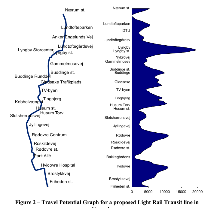
    - Left side represents the transit line.
    - Right Side
      - Y-Axis are locations where buffer areas were created.
      - X-Axis: Travel Potential
        
        Not sure if that is just smoothed line with a point estimate of Travel Potential at each location or how exactly those values are calculated.
        
        50m isn’t a large distance so maybe all the locations aren’t shown on the Y-Axis and the number of calculations produces an already, mostly, smooth line on it’s own.
        
        Partitioning a buffer zone into rings or some kind of interpolation could provided more granular estimates around the central buffer location.