Discrete Choice Models

Misc

AKA Random Utility or Choice Models
tl;dr:
- The Utility equation is the model equation.
  - Utility ($U$) is made up of Observed Utility ($V$) and Unobserved Utility ($\epsilon$).
  - (Total) Utility is the LHS of the model equation
  - Logit models are typically used to estimate utility as predicted logits.
    - The predicted probabilities are called Choice Probabilities
    - If the data is aggregated to the Market Level instead of the individual level, then the predicted logits are now called Market Shares.
  - Observed Utility is modeled using our data, and Unobserved Utility is the residual of that model.
  - The coefficients ($\beta$s) (log odds ratios) of the model are called Marginal Utilities.
- The observed response is typically polytomous and the categories are called Alternatives which are the potential choices of the Decision Maker.
Notes from ResEcon 703 Video Course
- Weeks 3, 4, 9, 10, 12, and 13
- Video lectures talk through mathematics (interpretations, motivations, benefits, limitations, etc.) of the approaches. Each week ends with a coding session illustrating the approaches that’s not included in the videos but is included in the slides.
  - The slides are updated with new material while the videos have not.
- github with slides and problem sets/solutions with R code. Slides provide a deeper introduction to the application the algorithms and the econometrics. Problem set solutions have similar material but written out more clearly. {mlogit} used throughout.
Also see:
- Decision Intelligence
- Regression, Multinomial
- Diagnostics, Classification >> Multinomial
- Algorithms, ML >> Discriminant Analysis >> Linear Discriminant Analysis (LDA)
- Model Building, brms >> Logistic Regression
Use Cases:
- Respondents to a social survey are classified by their highest completed level of education, taking on the values (1) less than highschool, (2) highschool graduate, (3) some post-secondary, or (4) post-secondary degree.
- Women’s labor-force participation is classified as (1) not working outside the home, (2) working part-time, or (3) working full-time.
- Voters in Quebec in a Canadian national election choose one of the (1) Liberal Party, (2) Conservative Party, (3) New Democratic Party, or (4) Bloc Quebecois.

Terms

Alternative - The levels of a polytomous response in Random Utility Models.
Choice Probability - The probability that a decision-maker will chose a particular alternative. The predicted response for a Random Utility Model.
Choice Settings - Can describe in general the choice set itself, or can also be used to describe the context in which the choice by the decision-maker is taking place.
- e.g. binary, ordered multinomial, unordered multinomial, and count data frameworks
- e.g. educational setting, marketing setting
- e.g. costs associated with each alternative for each individual
Consumer Surplus - Monetary gain to a consumer from “purchasing” a good for less than the value the consumer places on the good
Cost Trade-Offs - How changes in one in a choice attribute can be offset by another.
- e.g. If the operating cost were to increase by $1, what reduction the purchase price would result in the same utility/choice probability for the consumer.
Discounted Utility - The utility of some future event, such as consuming a certain amount of a good, as perceived at the present time as opposed to at the time of its occurrence. It is calculated as the present discounted value of future utility, and for people with time preference for sooner rather than later gratification, it is less than the future utility.
Marginal Utility - Coefficients in the logit model (log odds ratios). The added satisfaction that a consumer gets from having one more unit of a good or service. The concept of marginal utility is used by economists to determine how much of an item consumers are willing to purchase.
Market Level - Environment or category where a class or brand of products share the same attributes
- e.g. All Cokes should cost the same in Indianapolis but that price may be different from the price of Cokes in Nashville. Therefore, Indianapolis and Nashville are separate markets.
Market Share - The percentage of total sales in an industry or product category that belong to a particular company during a discrete period of time. For a Random Utility Model, when the data is at the market level instead of the individual level, the predicted response is the Market Share.
Outside Product (aka Outside Option) - Typically a “purchase nothing” indicator variable/variable category
- Can just be a vector of 0s
Random Utility Models - These models rely on the hypothesis that the decision maker is able to rank the different alternatives by an order of preference represented by a utility function, the chosen alternative being the one which is associated with the highest level of utility. They are called random utility models because part of the utility is unobserved and is modeled as the realization of a random deviate.

Random Utility Models

Misc
Random Utility - utility theory can readily be understood as the idea that people behave in line with self-interset where self-interest reflects peoples’ needs to save time and economize on effort.
- These models rely on the hypothesis that the decision maker is able to rank the different alternatives by an order of preference represented by a utility function, the chosen alternative being the one which is associated with the highest level of utility. They are called random utility models because part of the utility is unobserved and is modeled as the realization of a random deviate.
Data sets used to estimate random utility models have therefore a specific structure that can be characterized by three indexes: the alternative, the choice situation, and the individual. The distinction between choice situation and individual indexes is only relevant if we have repeated observations for the same individual.
- Examples of variable types
  - Data Descriptions
    - Each individual has responded to several (up to 16) scenarios.
    - For every scenario, two train tickets A and B are proposed to the user, with different combinations of four attributes: price (the price in cents of guilders), time (travel time in minutes), change (the number of changes) and comfort (the class of comfort, 0, 1 or 2, 0 being the most comfortable class).
  - Choice Situation Specific
    - data1: Length of the vacation and the Season
    - data2: values of dist, income and urban are repeated four times.
      - dist (the distance of the trip)
      - income (household income)
      - urban (a dummy for trips which have a large city at the origin or the destination)
      - noalt the number of available alternatives
  - Individual Specific
    - data1: Income and Family Size
    - data2: None
  - Alternative Specific
    - data1: Distance to Destination and Cost
    - data2:
      - transport modes (air, train, bus and car)
      - cost for monetary cost
      - ivt for in vehicle time
      - ovt for out of vehicle time
      - freq for frequency
- The unit of observation is typically the choice situation, and it is also the individual if there is only one choice situation per individual observed, which is often the case
Agent/Decison-Maker gets some amount of utility from each of the alternatives (set of actions the user can choose from)
The amount of utility for each alternative and each decision maker can depend on:
- observed characteristics of the alternative themselves
- observed characteristics of the decision maker
- unobserved characteristics
Utility is not observed but can be inferred by factors that are observed (and how each factor affects Utility):
- Chosen alternative, i, by each decision maker, n
- Some attributes about each alternative
- Some attributes about each decision maker.
Total Utility: $U_{nj} = V_{nj} + \epsilon_{nj}$
- Where Representative (or Observed) Utility, $V_{nj} = V(x_{nj}, s_n)$
  - $x_{nj}$ is the vector of attributes for alternative j specific to decison maker n
  - $s_n$ is the vector of attributes for decision maker n\
- $\epsilon_{nj}$ is called the “Random Utility” which is unobserved (i.e. the stuff we didn’t adjust for).
Utility Model: $U_{nj} = \hat{\beta}x_{nj} + \epsilon_{nj}$
- $V_j = \hat{\beta} \boldsymbol{x}$
- Since $U_{nj}$ is unobserved, decision maker choice from alternatives is used as the response variable to proxy Utility.
- $\beta$ is called a “structural parameter”
Choice Probabilities

\[ P_{ni} = \int_{\epsilon} \mathbb{1} (\epsilon_{nj} - \epsilon_{ni} < V_{ni} - V_{nj} \;\; \forall j \neq i) f(\boldsymbol{\epsilon}_n) d \boldsymbol{\epsilon}_n \]
- Assuming the decision maker makes choices that maximize utility allows us to use choice probabilities to model which alternative maximizes utility.
- See video for the derivation from $\text{PR}(U_{ni} > U_{nj} \;\; \forall j \neq i)$
- This is the cumulative distribution for $\epsilon_{nj} - \epsilon_{ni}$ which is a multidimensional integral over the density of unobserved utility, $f(\epsilon_n)$.
- Assumptions about $f(\epsilon_n)$ are what yields different discrete choice models

Binary Logit

Misc
Choice Probability

\[ \begin {align} P_{n1} &= \frac {1}{1 + e^{-(V_{n1} - V_{n0})}} \\ &= \frac{1}{1 + e^{-(\hat \beta \boldsymbol{x})}} \end {align} \]
- The probability of decision maker, $n$, selecting choice, $1$.
  - i.e. predicted probability
- The estimated utility of decision maker, $n$, selecting choice, $1$ is the predicted logit not the predicted probability
Cost Trade Offs
- See Terms
- Example: An increase in “operating cost” would need to be offset in how much of a reduction in purchasing price in order for the decision maker’s utility not to change?
  
  \[ \begin {align} U_{n1} &= \beta_0 + \beta_1 P_n + \beta_2 C_n + \epsilon_{n1} \\ dU_{n1} &= \beta_1 dP_n + \beta_2 dC_n \\ dU_{n1} &= 0 \implies \frac{dP_n}{dC_n} = -\frac{\beta_2}{\beta_1} \end {align} \]
- Also see Example: Preferences for Air Conditioning
Implied Discount Rate
- See Terms
- Example:
  
  \[ \begin {align} (1) \;\; U_{n1} &= \alpha_0 + \alpha_1(P_n + \frac{1}{\gamma}C_n) + \omega_n \\ (2) \;\; U_{n1} &= \beta_0 + \beta_1P_n + \beta_2C_n + \epsilon_{n1} \\ &\therefore \; \alpha_1 = \beta_1 \;\&\; \frac{\alpha_1}{\gamma} = \beta_2 \\ &\implies \gamma = \frac{\beta_1}{\beta_2} \end {align} \]
  - $P_n$ is product price and $C_n$ is the product’s operating cost
  - $\gamma$ is the discount rate
  - $\alpha_1$ is supposed to be the marginal utility for household income but it doesn’t play into the discount rate calculation
  - (1) is the general formula for a household’s expected utility after purchasing the product which assumes infinite time horizon for operating cost
  - (2) binary logistic model equation for utility
Example: Student preferences for either driving their car or riding the bus to campus
- Model
```
model_1a <- 
  glm(formula = car ~ cost.car + time.car + time.bus,
      family = 'binomial',
      data = data_binary)
```
  - car - TRUE/FALSE binary variable that indicates whether the decision maker chose to drive (TRUE) or take the bus (FALSE)
  - cost.car - continuous, cost (in dollars) to drive to campus
  - time.car - continuous, time (in minutes) to drive to campus
  - time.bus - time (in minutes) to ride the bus to campus
- summary Results
```
#> Coefficients:
#>             Estimate Std. Error z value Pr(>|z|)    
#> (Intercept)  2.23327    0.34662   6.443 1.17e-10 ***
#> cost.car    -2.07716    0.73245  -2.836  0.00457 ** 
#> time.car    -0.33222    0.03534  -9.400  < 2e-16 ***
#> time.bus     0.13257    0.03240   4.092 4.28e-05 ***
```
  - Coefficents (log ORs) are marginal utilities
  - The cost of driving and the time spent driving both decrease the utility of driving, and the time spent riding the bus increases theutility of driving relative to riding the bus.
  - Intercept: Driving a car generates 2.23 “utils” of utility
  - cost.car: Each additional dollar of driving cost reduces utility of driving by 2.08
  - time.car: Each additional minute of driving reduces utility of driving by 0.33
  - time.bus: Each additional minute riding on the bus increases utility of driving by 0.13
- The dollar value that a student places on each hour spent driving and on each hour spent on the bus.
```
## Calculate hourly time-value for each commute mode
abs(coef(model_1a)[3:4] / coef(model_1a)[2]) * 60
#> time.car time.bus
#> 9.596257 3.829494
```
  - Each hour of driving has a dollar value of $9.60 and each hour of bus riding has a dollar value of $3.83.
    - In other words, a student would be willing to pay $9.60 to spend one less hour commuting by car but only $3.83 to spend one less hour commuting by bus.
  - Since the time variables are in minutes, I would’ve guessed that you would divide by 60 to get hours. Dividing by 60 gives you values of only 1000^ths of a dollar though, so I guess not.
- Allowing cost to vary inversely by income (aka Heterogeneous Parameter)
```
model_1b <- 
  glm(formula = car ~ I(cost.car / income) + time.car + time.bus,
      family = 'binomial',
      data = data_binary)

summary(model_1b)
#> Coefficients:
#>                     Estimate Std. Error z value Pr(>|z|)    
#> (Intercept)          2.26541    0.33110   6.842 7.81e-12 ***
#> I(cost.car/income) -53.63314   14.54884  -3.686 0.000227 ***
#> time.car            -0.33521    0.03484  -9.622  < 2e-16 ***
#> time.bus             0.13589    0.02880   4.719 2.37e-06 ***
```
  - Dividing cost by income takes into account that students with different incomes might have different sensitivities to cost
    - income - student annual income (in 1000 dollars)
  - A higher level of income yields a lower marginal utility of cost.
  - Intercept: Driving a car generates 2.27 “utils” of utility
  - cost.car/income: An additional 0.1 percentage point of cost.car (i.e. driving cost) as a share of income reduces utility by -53.63
    - I think a “share” means that proportion of car.cost to income increases by 0.1 of a percentage point
  - Calculate marginal utility of car cost at different incomes
```
-coef(model_1b)[2] / c(15, 25, 35)
#> [1] 3.575543 2.145326 1.532375
```
    - He doesn’t give units when stating these results, but did so when taking the ratio of 2 marginal utilities.
    - He takes the negative here, but I’m not sure if that’s because you always take the negative or he’s just looking for the magnitude (i.e. abs).
      - I feel like it’s the latter. If that’s the case though, then it will always be the case that a larger income means less absolute marginal utility no matter the value of the coefficient.
      - So this seems that your making that assumption beforehand by choosing to divide by income instead of multiplying by it, and the goal is to just calculate the amounts by which the effect of cost is affected by larger incomes.
  - Calculate hourly time-value for each commute mode at different incomes
```
rep(abs(coef(model_1b)[3:4] / coef(model_1b)[2]), 3) * 
  c(rep(15, 2), rep(25, 2), rep(35, 2)) * 60
#> time.car  time.bus  time.car  time.bus  time.car  time.bus 
#> 5.625096  2.280260  9.375160  3.800433 13.125224  5.320607 
```
    - At each of these incomes, each hour of driving has a dollar value of $5.63, $9.38, and $13.13, respectively; and each hour of bus riding has a dollar value of $2.28, $3.80, and $5.32, respectively.
Example: Visualization
- Kernel Density of Estimated Utilities
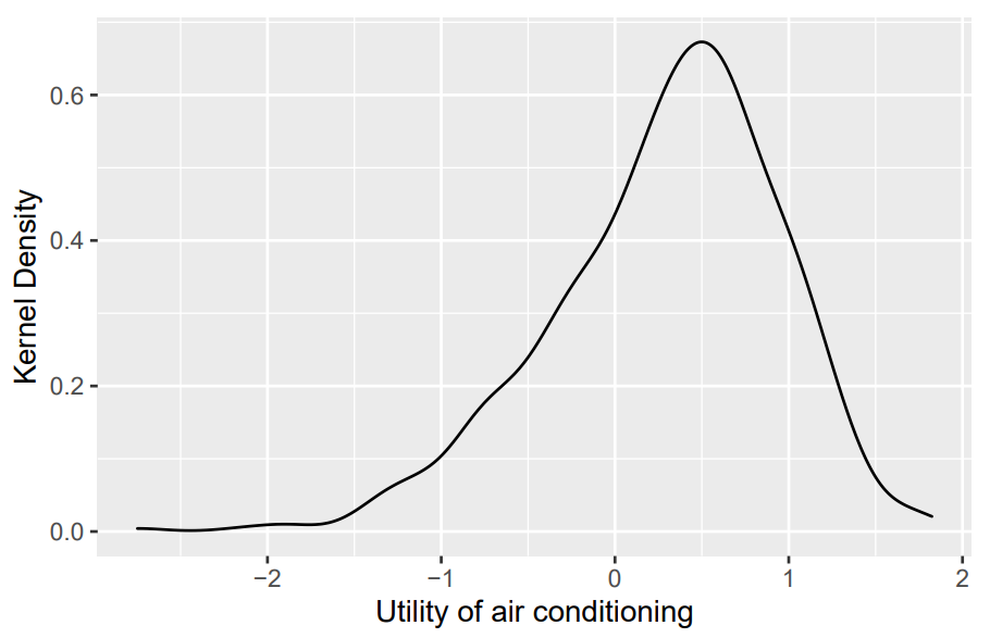
```
## Plot density of utilities
ac_data %>%
ggplot(aes(x = utility_ac_logit)) +
geom_density() +
xlab('Utility of air conditioning') +
ylab('Kernel Density')
```
  - Where utility_ac_logit = predict(binary_logit_mod)
    - Can also do this with choice probabilities
- Fraction of Choice (Adoption) vs Estimated Utility
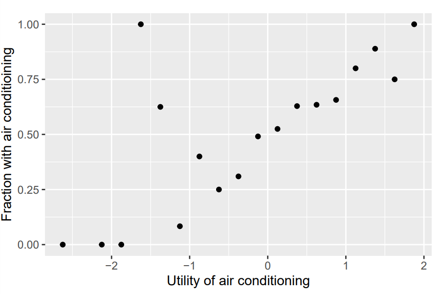
```
ac_data %>%
  mutate(bin = cut(utility_ac_logit,
                   breaks = seq(-3, 2, 0.25),
                   labels = 1:20)) %>%
  group_by(bin) %>%
  summarize(fraction_ac = mean(air_conditioning), .groups = 'drop') %>%
  mutate(bin = as.numeric(bin),
         bin_mid = 0.25 * (bin - 1) - 2.875) %>%
  ggplot(aes(x = bin_mid, y = fraction_ac)) +
    geom_point() +
    xlab('Utility of air conditioning') +
    ylab('Fraction with air conditioining')
```
  - From Week 4 slides at around slide 59
  - Shows the fraction of adoption of air conditioning (choice 1) within each bin of estimated utility.
    - Can also do this with choice probabilities
  - In general, we expect decision makers with greater estimated utility to choose air conditioning more often which is what is seen.
    - There are a couple of exception around bin -1.5, but maybe those are due to there not being enough individuals in those bins to be representative. Otherwise, the model is missing something for these individuals.
  - I’m not sure if this should be linear or maybe sigmoid — it’s a proportion vs a logit. Think I’m leaning towards sigmoid.
    - He did do this with choice probabilities and that one looked linear which is what you’d expect since it’s like a observed vs predicted plot.

Example: Marginal Effects and Elasticities

These formulas are the same as the ones shown in the Multiomial Logit section
These values are on the observation level so one useful thing to look at would be summary statistics and density plots

Marginal Effects

ac_data <- ac_data %>%
mutate(marg_eff_system = coef(binary_logit_mod)[2] *
          probability_ac_logit * (1 - probability_ac_logit),
       marg_eff_operating = coef(binary_logit_mod)[3] *
          probability_ac_logit * (1 - probability_ac_logit))

Elasticities

ac_data <- ac_data %>%
mutate(elasticity_system = coef(binary_logit_mod)[2] *
          cost_system * (1 - probability_ac_logit),
       elasticity_operating = coef(binary_logit_mod)[3] *
          cost_operating * (1 - probability_ac_logit))

Example: Preferences for Air Conditioning
- Model
```
binary_logit <- 
  glm(formula = air_conditioning ~ cost_system + cost_operating,
      family = 'binomial',
      data = ac_data)
```
  - air_conditioning: Binary TRUE/FALSE, the choice between buying an AC (TRUE) or not (FALSE)
  - cost_system: Cost of buying the AC
  - cost_operating: Cost of operating the AC
- Cost Trade-Offs
```
-coef(binary_logit)[3] / coef(binary_logit)[2]
## cost_operating
## -5.186972
```
  - Says a dollar increase in AC purchasing cost would need to be offset by a decrease of $5.19 in operating cost in order for the customer utility for buying an AC to remain the same.
- Implied Discount Rate
```
coef(binary_logit)[2] / coef(binary_logit)[3]
## cost_system
## 0.1927907
```

Multinomial Logit (MNL)

See Regression, Multinomial >> Multinomial Logit for examples
AKA Generalized Logit
When the polytomous response has m levels (aka Alternatives), the multinomial logit model comprises m−1 log-odds comparisons with a reference level, typically the first or last.
- The likelihood under the model and the fitted response probabilities that it produces are unaffected by choice of reference level, much as choice of reference level for dummy regressors created from a factor predictor doesn’t affect the fit of a regression model.
Choice Probability for alternative, i, and decision-maker, n:

\[ P_{ni} = \frac {e^{V_{ni}}}{\sum_j e^{V_{nj}}} = \frac {e^{\hat{\beta}x_{ni}}}{\sum_j e^{{\hat{\beta}x_{nj}}}} \]
- The probability that decision-maker, $n$, chooses alternative, $i$
- Predicted probability output from the model
Market Shares
- Market Share for alternative, i
  
  \[ S_i = \frac {e^{V_i}}{\sum_j e^{V_j}} \]
  - What distinguishes this from a choice probability is that unit is at the market level and not the individual level (see $\vec{x}$ in the next section), hence no “n” in the equation
- The difference in market share of products i and j
  
  \[ \ln (S_i) - \ln (S_j) = \hat{\beta} (x_i - x_j) \]
  - $x_i$ is a set of variables that describe product i.
    - Therefore these will be the same for every decision-maker.
  - $j$ is typicially a reference level (aka outside option)
    - If the products were a product such as cereal, then the outside option would typically be “not buying cereal” where the utility is 0.
Consumer Surplus
- The expected consumer surplus that decision maker n obtains when faced with a choice setting is
  
  \[ \nabla \mathbb{E}(CS_n) = \frac{1}{\alpha_n} \left[\ln \left(\sum_{j=1}^{J^1} e^{V^1_{ng}} \right) - \ln \left(\sum_{j=0}^{J^1} e^{V^0_{ng}} \right) \right] \]
Assumptions
- Exogenity of the alternative attribute variables of the alternatives: $\mathbb{E}[\epsilon \; | \; \vec {x}] = 0$ (i.e mean of the residuals is 0)
  - Example of Endogenity
    - Taking a car to work or taking the bus to work are the alternatives.
    - If a commuter likes to drive, they won’t care about living close to a bus stop
    - If a commuter likes to take the bus, they are more likely to live close to a bus stop
    - Therefore your logit model will be biased because any attribute variable that is related to the distance a decision-maker is from a bus stop will be endogenous.
      - e.g. Time each mode of transportation takes to get to work will be endogenous because distance from the bus stop affects time and distance to bus stop is correlated with a decision maker already biased towards buses and not with a decision maker who would choose bus or car.
        
        i.e. distance isn’t randomly distributed among all decision makers.
  - Solution: TBD in a later lecture
- iid residuals following a Gumbel distribution
  - Residuals are the unobserved utility (i.e. random utility).
  - For panel data, it’s unlikely that each unobserved alternative attribute for a decision maker is independent across a time component which makes this a bad model for such data.
    - e.g. If a person chooses Count Chocula one day and Fruit Loops the next, it’s unlikely that the unobserved components of utility that led to the Count Chocula choice aren’t correlated with the unobserved components of utility that led to the Fruit Loops choice.
Substitution Patterns
- Independence of Irrelavent Alternatives (IIA) Property of Logit models
  - Example: car, blue bus , red bus
    - In the beginning, the decision maker only has 2 choices: drive car or ride blue bus.
    - The probability of choosing the alternative car is the same for a decision maker as choosing the alternative blue bus: $P_c = P_{bb} = 1/2$
    - Then a red bus is added to the choices, but the decision maker doesn’t care whether the bus is red or blue. Therefore the blue bus and the red bus have the same choice probability: $P_{bb} = P_{rb}$
    - But from the IIA property, the ratio of choice probability between car and blue bus is not changed after introduction of the red bus. Therefore, $P_c = P_{bb} = P_{rb} = 1/3$
    - In reality, the choice probability for car has NOT decreased, since for decision maker, the choice is actually between car and bus — color isn’t a relative factor
  - Example: Hummer, Escalade, Prius
    - Hummer lowers price.
    - Will Hummer attract more Escalade drivers than Prius?
    - The logit model says that “proportional substitution to the Hummer will be equal for the Escalade and the Prius.
      - i.e. The lowering of the Hummer price will have an equal effect on Escalade sales and Prius sales which is unrealistic
- Proportional Substitution
  - Note the logit cross-elasticity equation for alternative, i, given a change in alternative, j (See below, Elasticity >> Cross Elasticity). The change in choice probability for alternative i only depends on the change to the attribute for alternative, j.
  - This means that we can substitute any alternative for i (other than j) and the cross-elasticity will be the same and therefore the change in choice probability will be the same.
    - i.e. We change the value of an attribute for alternative j. Then, all choice proabilities for the other alternatives (other than j) change by the same proportion. Doesn’t matter if alternative j is correlated more strongly with another alternative or not.
  - Shows a lack of flexibility in the logit model — there is no structure to model the correlation between alternatives. (See Mixed Logit)
Marginal Effects

\[ \text{ME} = \frac {\partial P_{ni}} {\partial z_{ni}} = \beta_z P_{ni}(1-P_{ni}) \]
- The change in the probability of choosing alternative, i, after a change in the attribute of alternative, i.
- $P_{ni}$ is the probability of decision maker, n, choosing alternative i.
- Cross Marginal Effect \[ \text{CME} = \frac {\partial P_{ni}} {\partial z_{nj}} = -\beta_z P_{ni}P_{nj} \]
  - The change in the probability of choosing alternative, $i$, after a change in the attribute of alternative, $j$.
Elasticity

\[ E_{iz_{ni}} = \beta_z z_{ni} (1-P_{ni}) \]
- Marginal Effects and Elasticities are similar except elasticities are percent change.
  - e.g. a percentage change in a regressor results in this much of a percentage change in the response level probability
- $E_{iz_{ni}}$ is the elasticity of the probability of alternative, i, with respect to $z_{ni}$, an observed attribute of alternative, i
- $P_{ni}$ is the predicted probability of alternative, i, for decision maker, n.
- Cross Elasticity \[ E_{iz_{ni}} = -\beta_z z_{nj} P_{nj} \]

Nested Logit

Fits separate models for each of a hierarchically nested set of binary comparisons among the response categories. The set of m−1 models comprises a complete model for the polytomous response, just as the multinomial logit model does.
Misc
- IIA still holds for two alternatives in the same dichotomy, but doesn’t hold for alternatives of different different dichotomies
- Both MNL and Nested Logit methods have have p×(m−1) parameters. The models are not equivalent, however, in that they generally produce different sets of fitted category probabilities and hence different likelihoods.
  - Multinomial logit model treats the response categories symmetrically
- Extensions
  - Paired Combinatorial Logit
    - Allows alternatives to be in multiple dichotomies and multiple hierarchies and for them to have more complex correlation structures
      - In nested logits, only alternatives within the same hierarchy are modeled as being correlated with each other.
    - Creates pairwise dichotomies for each combination of alternatives (i.e. each alternative appears in J-1 nests)
    - Best for data with fewer alternatives since the parameter space can explode fairly quickly
  - Generalized Nested Logit
    - Allow alternatives to be in any dichotomy in any hierarchy, but assign a weight to each alternative in each dichotomy.
    - Estimate Parameters: $\lambda_k$ (See Choice Probability below), $\alpha_{jk}$ : “weight” or proportion of alternative, $j$, in dichotomy, $k$
    - Need to be careful about how many dichotomies that you place each alternative, since the parameter space can explode fairly quickly
  - Heteroskedastic Logit
    - Heteroskedacity in this sense means that the variance of the unobserved utility (aka residuals) can be different for each alternative
      
      \[ \mbox{Var}(\epsilon_{nj}) = \frac {(\theta_j \pi)^2}{6} \]
    - Since there’s no closed form solution, simulation methods must be usded to get the choice probabilities and model parameters.
Construction of Dichotomies
- By the construction of nested dichotomies, the submodels are statistically independent (because the likelihood for the polytomous response is the product of the likelihoods for the dichotomies), so test statistics, such as likelihood ratio (G²) and Wald chi-square tests for regression coefficients can be summed to give overall tests for the full polytomy.
- Nested dichotomies are not unique and alternative sets of nested dichotomies are not equivalent: Different choices have different interpretations. Moreover, and more fundamentally, fitted probabilities and hence the likelihood for the nested-dichotomies model depend on how the nested dichotomies are defined.
- Example: 2 methods of splitting a 4-level response into dichotomies
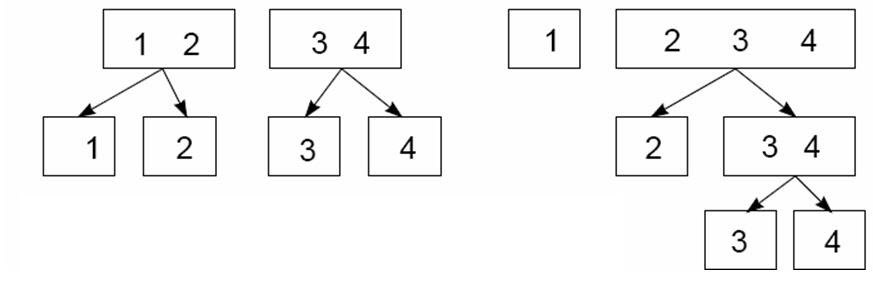
  - Left: Y = {1, 2, 3, 4} → {1,2} vs {3,4} → {1} vs {2} and {3} vs {4}
  - Right: (Continuous Logit) Y = {1, 2, 3, 4} → {1} vs {2, 3, 4} → {2} vs {3, 4} → {3} vs {4}
    - {1} vs. {2,3,4} could represent highschool graduation
    - {2} vs. {3,4} could represesnt enrollment in post-secondary education
    - {3} vs. {4} could represent completion of a post-secondary degree.
Assumptions
- Assumes Gumbel distribution of errors but relax the i.i.d. hypothesis
  - Allows for the unobserved (and random) components of utility, $\epsilon_{nj}$ , to be correlated for the same decision maker
  - Example: {drive} vs {carpool} and {bus} vs {train}
    - Model allows from unobserved components of utility (i.e. residuals of the model) of drive and carpool to correlated for the same decision maker but not the unobserved components of utility for carpool and train.
- Assumes Exogenity (See Multinomial Logit >> Assumptions)
  - This model is also bad for panel data
Choice Probability for alternative, i, and decision-maker, n

\[ P_{ni} = \frac {e^{V_{ni}/\lambda_k}(\sum_{j\in B_k}e^{V_{nj}/\lambda_k})^{\lambda_k - 1}}{\sum_{\ell=1}^K (\sum_{j\in B_\ell}e^{V_{nj}/\lambda_\ell})^{\lambda_\ell}} \]
- The probability that decision-maker, $n$, chooses alternative, $i$
  - Predicted probability output from the model
  - When data is at the market level, the $n$ index (i.e. individual) is removed from the equation above and the LHS becomes Market Share (See Terms). The difference in market share between alternatives (e.g. brands) is:
    
    \[ \ln(S_i) - \ln(S_m) = \hat{\beta}(x_i - x_m) + (1-\lambda_k)\ln S_{i|B_k} - (1-\lambda_\ell)S_{m|B_\ell} \]
    - The index, $m$, is typically a reference level called the “outside option” (See Terms) which is alternative of NOT doing an action where the utility is 0.
      - If the products were a product such as cereal, then the outside option would typically be “not buying cereal” which would have a utility is 0.
- $\lambda_k$ is a measuer of independence in dichotomy, $k$ that gets estimated
- $1-\lambda_k$ is a measure of the correlation within dichotomy, $k$
- The nested logit is consistent with the random utility model when $\lambda_k \in (0,1] \; \forall k$
Elasticity

\[ E_{iz{ni}} = \beta_z z_{ni} \left(\frac{1}{\lambda_k} - \frac{1-\lambda_k}{\lambda_k}P_{ni|B_k} - P_{ni}\right) \]
- Marginal Effects and Elasticities are similar except elasticities are percent change.
  - e.g. a percentage change in a regressor results in this much of a percentage change in the response level probability
- Elasticity of alternate, $i$, in dichotomy, $k$, for decision-maker, $n$, with respect to its attribute, $z_{ni}$
Cross-Elasticity

\[ E_{iz_{nm}} = \left\{ \begin{array}{lcl} -\beta_z z_{zm}P_{nm} \left(1+ \frac{1-\lambda_k}{\lambda_k} \frac {1}{P_{nB_k}} \right) & \mbox{if} \; m \in \beta_k \\ -\beta_z z_{zm}P_{nm} & \mbox{if} \; m \notin \beta_k \end{array}\right. \]
- Where
  
  \[ P_{nB_k} = \sum \limits_{j \in B_k} P_{nj} \;\; \text{and} \;\; P_{ni|B_k} = \frac {P_{ni}}{P_{nB_k}} = \frac {P_{ni}}{\sum_{j \in B_k} P_{nj}} \]
- The percent change in the probability of choosing alternative, $i$, after a percent change in the attribute of alternative, $m$.
- Cross elasticity depends on whether both alternatives are in the same dichotomy.

Mixed Logit

Individual heterogeneity can be introduced in the parameters associated with the covariates entering the observable part of the utility or in the variance of the errors.
- Doesn’t exhibit IIA (See Multinomial Logit >> Substitution Patterns) since correlations between alternatives are modeled.
- Model creates a distribution of $\beta$s, so $\beta$ is allowed to vary throughout a population.
Misc
- Market Level Data
  - Observe price, market share, and characteristics of a product
Choice Probability

\[ \begin{align} &P_{ni} = \int L_{ni}(\beta) \; f(\beta\;|\;\boldsymbol{\theta}) \; d\beta\\ &\mbox{where} \; L_{ni}(\beta) = \frac {e^{V_{ni}(\beta)}}{\sum_{j=1}^J e^{V_{ni}(\beta)}} \end{align} \]
- $\boldsymbol{\theta}$ is a vector of distributional parameters (e.g. $\mu, \sigma^2$ for a Normal Distribution)
  - The $\theta$ parameters are what get estimated by the model in order to calculate a distribution of $\beta$s (i.e. Bayesian posterior)
- Integrates over a density so there is not a closed form solution. Therefore, numerical simulation must be used.
  - Elasticities don’t have a closed form solution either (Assume Marginal Effects are the same way)(See lecture videos for the math)
- Think of it as a weighted average of logit choice probabilities
  - The logit choice probabilities are evaluated a different values of $\beta$, and each logit choice probability is weighted by the density $f(\beta\;|\;\boldsymbol{\theta})$
    - i.e. Based on the density, more likely $\beta$s will be more heavily weighted.
- In statistical language, it’s a mixed function of logit choice probabilities, $L_{ni}(\beta)$, and the mixing distribution, $f(\beta\;|\;\boldsymbol{\theta})$
Random Coefficients

\[ U_{nj} = \hat{\alpha}\boldsymbol{x}_{nj} + \hat{\mu}\boldsymbol{z}_{nj} + \epsilon_{nj} \]
- $x_{nj}$, $z_{nj}$ - Data for alternative j and decision maker n
- $\hat{\alpha}$ - Vector of fixed coefficients (i.e. same for all decision makers)
- $\hat{\mu}_n$ - Vector of random coefficients (i.e. a coefficient for each decision maker)
- $\epsilon_{nj}$ - Residual from an extreme value distribution (e.g. Gumbel)
- Correlated Random Utility
  - Let $\nu_{nj} = \boldsymbol{\hat{\mu}}_n \boldsymbol{z}_{nj} + \epsilon_{nj}$ be the random (unobserved) component of utility and $\mbox{Cov}(\nu_{ni}, \nu_{nj}) = \boldsymbol{z}_{ni} \Sigma \boldsymbol{z}_{nj}$ the covariance between random utilities of different alternatives where $\Sigma$ is the variance/covariance matrix for $\boldsymbol{\hat{\mu}}$
  - This is a structure to model the correlation between alternatives
Panel Data
- Data where each decision maker makes multiple choices over time periods
- Model allows for unobserved preference variation through random coefficients, which yields correlations in utility over time for the same decision maker
- Decision maker, n, chooses from a vector of alternatives over T time periods
- Utility
  
  \[ U_{njt} = \hat{\beta}_n x_{njt} + \epsilon_{njt} \]
  - The utility, U, for decision maker, n, in choosing alternative, j, at time period, t.
  - $\hat{\beta}$ varies for each decision maker but is constant across time.
- Lag or lead predictors can be included
- Lagged responses can be included
  - Use cases:
    - Habit Formation
    - Variety-Seeking Behavior
    - Switching Costs
    - Brand Loyalty
- Only models a sequence of static choices
  - Lagged responses account for past choices affecting current choices, but not how current choices affect future choices
  - A fully dynamic discrete choice model models how every choice affects subsequent choices.
Individual-level Coefficients
- Conditional Distribution of Coefficients: $h(\beta \;|\; \boldsymbol{y}_n, \boldsymbol{x}, \boldsymbol{\theta})$
  - Distribution of $\beta$ among the group, from a popuation with an unconditional distribution defined by $\boldsymbol{\theta}$, who choose a sequence of alternatives $y_n$ when faced with choice setting, $\boldsymbol{x}$
  - $y_n$ is the sequence of choices made by decision maker, n (i.e. panel data)
  - $\boldsymbol{\theta}$ is the vector of $\beta$ distribution parameters
  - $\boldsymbol{x}$ is the vector of choice attributes
  - Proportional to the product (i.e. joint distribution) of
    
    \[ P(\boldsymbol{y}_n \;|\; \boldsymbol{x}_n, \beta) \;\times\; f(\beta \;|\; \boldsymbol{\theta}) \]
    - (Left) The probability that an individual with coefficients $\beta$ would choose $y_n$
    - (Right) The likelihood of observing $\beta$ in the population
- Mean of the Conditional Distribution (aka Conditional Mean Coefficients)
  - More practical to calculate than the conditional distribution itself.
  - It’s the weighted average of vectors of $\beta$ drawn randomly from the $\beta$ distribution, $\text f(\beta|\boldsymbol{\theta})$, $R$ times.
    
    \[ \begin {align} \breve{\beta}_n &= \sum_{r=1}^R w_r \beta_r \\ \mbox{where} \;\; w_r &= \frac{P(\boldsymbol{y}_n|x_n, \boldsymbol{\beta}_r)}{\sum_{r=1}^R P(\boldsymbol{y}_n|x_n, \boldsymbol{\beta}_r)} \end {align} \]
    - $w$ is the weight which is the proportion choice probability for draw, $r$
  - A decision maker must make many choices for the conditional mean coefficient to approach the true individual-level coefficient.
    - A Monte Carlo simulation in the textbook for these lectures said even after 50 choices there was substantial difference between the two values. Although, in the era of big data, it is conceivable to see a person make hundreds of choices.
- Future Choice Probabilities
  - Use past choices to define a conditional distribution of coefficients for the decision-maker
  - Then use this conditional distribution, instead of the unconditional distribution, to calculate the mixed logit choice probabilities.
    - No closed form solution so must use simulation. See lecture video for the procedure, but it’s similar to the procedure of the conditional mean coefficient above.

Dynamic Discrete Choice Models

Unlike the previous static models , this model will explicitly represent how 1 choice affects future choice sets and therefore future utilities.
- Static models assume that you make a choice based on the utility of that choice alone at that current time and not on some future utility associated with that first choice.
Utility
- Two Examples for “Go to college or get a job”
  - Total Utility for:
    - Two Periods: The utility gained during 4 years of college or work + the utility gain by choosing a job from a job set that depends on the completion of college or working for 4yrs
    - Three Periods: Same as two but add in utility gained after choosing a retirement plan from a set of plans that were determined by the job you chose in period 2.
  - Decision maker attends college $\; iff \;\; TU_C > TU_W$
  - 2 Period Setting: During College/Work and Available Jobs After College/Work
    
    \[ \begin {align} TU_C &= U_{1C} + \lambda \max_j (U_{2j}^C) \\ TU_W &= U_{1W} + \lambda \max_j (U_{2j}^W) \end {align} \]
    - College ($C$) or Work ($W$) for four years
    - $U_1C$ - Utility in period 1 from four years of college
      
      \[ U_{1C} = V_{1C} + \epsilon_{1C} \]
    - $U_1W$ - Utility in period 1 from four years of working (Similar equation to $U_{1C}$ )
    - $U_{2j}^C$ - Utility in period 2 from job $j$ after attending college
      
      \[ U_{2j}^C = V_{2j}^C + \epsilon_{2j}^C \]
    - $U_{2j}^W$ - Utility in period 2 from job $j$ after working (Similar equation to $U_{2j}^C$ )
    - $\max$ says the person will take whichever job that gives the most utility
      - Job choice set is different for decision makers who went to college than those that chose to work in the 1st period (even though both indexed by js).
    - $\lambda$ reflects relative weighting of the two periods. Factor that
      “discounts” a future utility. Typically people assign more utility for current things than things in the future, so in that case, this factor will lessen utility.
  - 3 Period Setting: Before College, After College, and Start of Retirement
    
    \[ \begin {align} TU_C &= U_{1C} + \lambda \max_j [U_{2j}^C + \theta \max_s (U_{3s}^{Cj})] \\ TU_W &= U_{1W} + \lambda \max_j [U_{2j}^W + \theta \max_s (U_{3s}^{Wj})] \end {align} \]
    - $J$ possible jobs for a career over many future years
    - $S$ possible retirement plans
      - $U_{3s}^{Cj}$ - Utility in period 3 from retirement plan $s$ after attending college in period 1 and working job $j$ in period 2
        
        Similar utility model equations as $U_{1C}$ and $U_{2j}^C$
      - $U_{3s}^{Wj}$ - Utility in period 3 from retirement plan $s$ after working in period 1 and working job $j$ in period 2
    - $\max$ is maximizing both job choice (period 2) and its associated retirement plan (period 3)
    - $\theta$ - Reflects relative weighting of three periods. Discount factor that’s the similar to $\lambda$.
Notation
- $\{i_1, i_2, \ldots, i_t\}$ - Sequence of choices up to and including period $t$
- $U_{tj}(i_1, i_2, \ldots, i_{t-1})$ - Utility obtained in period $t$ from alternative $j$, which depends on all previous choices
- $TU_{tj}(i_1, i_2, \ldots, i_{t-1})$ - Total Utility (current and all future time periods) obtained from choosing alternative $j$ in period $t$, assuming the optimal choice is made in all future periods. (aka Conditional Value Function) (i.e. conditional on the alternative)
  - All possible values of $TU_{tj}(i_1, i_2, \ldots, i_{t-1})$ need to be calculated in order to express the optimal choice in each time period
- $TU_t(i_1, i_2, \ldots, i_{t-1})$ - Total Utility obtained from the optimal choice in period $t$, assuming the optimal choice is made in all future periods (aka Value Function or Valuation Function at time $t$ )
  - $TU_t(i_1, i_2, \ldots, i_{t-1}) = \max_j TU_{tj}(i_1, i_2, \ldots, i_{t-1})$
Bellman Equation
- Incorporates Discounted Utility (See Terms) into the Value Functions
  - Generalization of the 2 “college or work” examples above and gives a procedure for how one would go about calculating the utilities for each period.
- Value Functions
  - Conditional Value Function
    
    \[ TU_{tj}(i_1, \ldots, i_{t-1}) = U_{tj}(i_1, \ldots, i_{t-1}) + \delta\max_k[TU_{t+1,k}(i_1, \ldots, i_t = j)] \]
    - Regarding $TU_{t+1}$, since $(i_1, \ldots, i_{t-1})$ says “given the sequence of choices prior to time, $t$,” the appending of $i_t = j$ is saying “given all the sequence of choices prior to time $t$ and includeing the current period, $t$, where choice $j$ is made.”
    - Not sure what $k$ is and he didn’t say in the video.
  - Value Function
    
    \[ TU_{t}(i_1, \ldots, i_{t-1}) = \max_j[U_{tj}(i_1, \ldots, i_{t-1}) + \delta\;TU_{t+1}(i_1, \ldots, i_t = j)] \]
    - Says that the total utility for time period $t$ i
    - $\delta$ - discount rate on utility in future periods (See Terms)
- Procedure: Work backwards from the last period to the first period to calculate the overall Total Utility. At each period (except the last period), you are using the utility calculated for the future period directly after it.
- Assumptions
  - Perfect information about:
    - Utility of each alternative in each future time period
    - How every possible sequence of choices affects this future utility
- With J alternatives in each of T time periods, you have to calculate $J^T \times T$ utilities.
  - Therefore, only model only broad time periods (e.g. [college, graduation, retirement]) in order to reduce the computational burden of calculating all these utilities.

Endogeneity

Need exogenous variation in our explanatory variables in order to give our parameter estimates a “causal” inerpretation
- If data are endogenous, our parameters can be interpreted as a kind of correlation between the data and choices
- True exogenous variable are tough to come by
Examples of Endogeneity
- Housing choice and commute choice are correlated
  - People who like public transit live closer to transit stations which makes their travel time lower
  - Therefore, the coefficient on travel time will be biased upwards
- Price and unobserved quality are correlated
  - Products with higher unobserved quality cost more and are preferrred by customers
  - Therefore, the coefficient on price with be biased downward and may even have the wrong sign
- Price and unobserved marketing are correlated
  - Large marketing campaigns may be accompanied by sales or increased prices (increased demand $\rightarrow$ decreased supply $\rightarrow$ increased price)
  - Therefore, the coefficient on price will be biased, but the direction is uncertain.
Solutions
- BLP estimation
- Control Function estimation
  - When to use Control Functions instead of BLP
    - If any market shares are zero
      - Constant terms in BLP are not identified for zero market shares
    - If you need to control for individual-specific endogeneity rather than market-level endogeneity (not feasible in BLP)
    - If you don’t want to use the Contraction Mapping algorithm.
      - More complex to code, computationally intensive
- Both methods use instruments
  - Good Instruments:
    - Correlated with explanatory variables
    - Exogenous (i.e. uncorrelated with residuals aka random utility aka unobserved utility)
  - Instruments are very context specific. So in order to find good instruments for your context, you need to know the details about the process you’re trying to model.

BLP (Berry-Levinsoln-Pakes)

Uses instruments to isolate exogenous variation in explanatory variables
Mixed logit model of demand for a differentiated product using market-level data.
- i.e. Estimate how the attributes of a product affect consumer demand
Price is one of the most important attributes, but is almost certainly correlated with other unobserved attributes
Model includes instruments in a nonlinear model
Utility Model
- If consumers also get utility from unobserved attributes, then Price is correlated with the composite error term ($\xi_{jm} + \epsilon_{njm}$)
- Therefore observed utility, $V$, gets separated into 2 componets, Consumer and Market.
  
  \[ \begin {align} U_{njm} &= \delta_{jm} + \tilde V (p_{jm}, \boldsymbol{x}_{jm}, \boldsymbol{s}_n, \boldsymbol{\tilde \beta}_n) + \epsilon_{njm} \\ \mbox where \;\; \delta_{njm} &= \bar V (p_{jm}, \boldsymbol{x}_{jm}, \boldsymbol{\bar \beta}_n) + \xi_{jm} = \bar{\hat{\boldsymbol{\beta}}}(p_{jm}, \boldsymbol{x}_{jm}) + \xi_{jm} \end {align} \]
  - $\tilde V (p_{jm}, \boldsymbol{x}_{jm}, \boldsymbol{s}_n, \boldsymbol{\tilde \beta}_n)$ - Component that varies by consumer
  - $\bar V (p_{jm}, \boldsymbol{x}_{jm}, \boldsymbol{\bar \beta}_n)$ - Component that varies by products and markets
  - $\delta_{jm}$ - Effectively becomes a product-market constant term (i.e. intercept that varies by product and market for a Mixed Logit model) that represents the average utility obtained by product $j$ in market $m$
    - This term gets estimated in the top equation. Then, this $\hat{\delta}$ is used as the LHS to estimate $\bar{\hat{\boldsymbol{\beta}}}$
  - $p_{jm}$ - Price of product $j$ in market $m$
    - 1 product can be the “outside product” or purchase nothing category (See Terms) which could be a vector of 0s
  - $\boldsymbol{x}_{jm}$ - Vector of non-price attribtuies of product $j$ in market $m$
  - $\boldsymbol{s}_n$ - Vector of demographice characteristics of consumer $n$
  - $\boldsymbol{\beta}_n$ - Vector of coefficients for consumer $n$
  - $\xi_{jm}$ - Utility (average) of unobserved attributes of product $j$ in market $m$
  - $\epsilon_{njm}$ - idiosyncratic (i.e. different per consumer) unobserved utility
  - The Choice Probability equation for this model looks similar to the Mixed Logit choice probability equation (See lecture video for the math)
Procedure
- Estimate the average utility for product $j$ in market $m$, including observable and unobservable attributes (top equation)
- Regress this average utilitiy value, $\hat{\delta}$, on price, $p_{jm}$, and other observable attributes, $x_{jm}$, while instrumenting for price. (i.e. IV model)
Issue
- $\hat{\delta}_{jm}$ must be estimated for each product in each market. This can result in 100s or even 1000s of terms to estimate.
BLP insights
- A set of unique $\delta_{jm}$ terms equates predicted market shares with observed market shares for a given set of $\boldsymbol{\theta}$ parameters
  - Higher $\delta_{jm}$ means there will be higher market shares for product $j$ in market $m$
- Their “Contraction Mapping” algorithm effectively finds these unique $\delta_{jm}$ terms
Contraction Mapping Algorithm
1. Start with initial value, $\delta^0$
2. Predict the market share for the current constant value, $\hat{S}_{jm}(\boldsymbol{\delta}^s)$, for each product and each market
  - $\hat{S}_{jm}(\boldsymbol{\delta})$ is the predicted market share (which is a function of delta)
    - I think these should be the predicted values for the Utility model above except the choice probabilities are now market shares since we’re predicting with market-level explanatory variables
  - The $s$ in the $\delta^s$ term seems to be a counter for which iteration of this algorithm that you’re on.
3. Adjust each product-market constant term by comparing predicted and observed market share
  
  \[ \delta_{jm}^{s+1} = \delta_{jm}^s + \ln \left(\frac{S_{jm}}{\hat{S}_{jm}(\boldsymbol{\delta}^s)}\right) \]
  - i.e. We’re adjusting our $\delta$ by the difference of log predicted and log observed market shares
4. Repeat steps 2 and 3 until the algorithm converges to the unique set of $\hat\delta$ (product-market) constants
  - Since this is a unique set, I think algorithm has converged with the observed market shares equal the predicted market shares exactly.
Overall Procedure
1. Outer-Loop: Search over $\boldsymbol{\theta}$ to optimize the estimation objective function
  - Inner-Loop: Use contraction mapping to find $\boldsymbol{\delta(\theta)}$, the vector of product-market constant terms conditional on $\theta$
  - Use $\boldsymbol{\theta}$ and $\boldsymbol{\delta(\theta)}$ to simulate choice probabilities, $P_{njm}(\boldsymbol{\delta(\theta)}, \boldsymbol{\theta})$
  - Use the choice probabilities to calculate the estimation objective function
2. Estimate $\boldsymbol{\bar\beta}$ by regressing $\boldsymbol{\delta_{jm}}$ on $(p_{jm}, \boldsymbol{x}_{jm})$ with price instruments, $\boldsymbol{z}_{jm}$
Estimator Options (See Week 13, video 5 lecture for details)
- Maximized Simulated Likelihood (MSL) for step 1 and Two-Stage Least Squares (2SLS) for step 2
- MSM - Some kind of method of moments algorithm
  - Method of Moments Characteristics (link)
    - Existence of Moments: Up to a certain order is necessary and requires finite tails in the distribution of the data.
    - Correct Model Specification: The underlying model must be correctly specified, including the functional relationship and the distribution of error terms.
    - Identifiability: There must be a unique solution for the parameters to be estimated.
    - Moment Conditions: It is necessary to specify the moment conditions correctly, which must have zero mean under the model assumptions.
    - Valid Instruments: If applicable, instruments must be relevant and valid.
    - Independence and Homoscedasticity (conditional): Ideally, errors should be independent and homoscedastic under the moment conditions.
    - Robustness to Heteroscedasticity: GMM is robust to heteroscedasticity if the weighting matrix is consistently estimated.
    - Multicollinearity: GMM can handle multicollinearity, but it can affect the efficiency of the estimators.
    - Outliers: GMM is sensitive to outliers unless they are properly addressed in the modeling process.
    - Large Samples: GMM is more efficient in large samples.
    - Asymptotic Theory: Properties such as consistency and efficiency are asymptotic.

Control Function

Use instruments to control for endogeneity in explanatory variables
Utility Model

\[ \begin {align} U_{nj} &= V(y_{nj}, \boldsymbol{x}_{nj}, \boldsymbol{\beta}_n) + \epsilon_{nj} \\ \\ \mbox{where} \;\; y_{nj} &= W(\boldsymbol{z}_{nj}, \boldsymbol{\gamma}) + \mu_{nj} \\ \epsilon_{nj} &= CF(\mu_{nj}, \boldsymbol{\lambda}) + \tilde \epsilon_{nj} \\ CF(\mu_{nj}, \boldsymbol{\lambda}) &= \mathbb{E}[\epsilon_{nj} \;|\; \mu_{nj}] \end {align} \]
- $y_{nj}$ - Endogenous explanatory variable (e.g price) for consumer $n$ and product $j$
- $\boldsymbol{x}_{nj}$ - Vector of non-price attributes for consumer $n$ and product $j$
- $\boldsymbol{\beta}_n$ - Vector of coefficients for consumer $n$
  - Has density, $f(\boldsymbol{\beta}_n,\boldsymbol{\theta})$
- $\epsilon_{nj}$ - Unobserved utility for consumer $n$ and product $j$ (i.e. residuals)
- $\tilde \epsilon_{nj}$ - The leftover unobserved utility that is not correlated with $\mu_{nj}$
  - Has the conditional density $g(\tilde \epsilon_n, \boldsymbol{\mu_n})$
  - This term controls for the source of endogeneity and therefore $y_{nj}$ is no longer endogenous.
- $\boldsymbol{z}_{nj}$ - Vector of exogenous instruments for $y_{nj}$
- $\boldsymbol{\gamma}$ - Parameters that relate $y_{nj}$ to $\boldsymbol{z}_{nj}$
- $\mu_{nj}$ - Unobserved factors that affect $y_{nj}$ (i.e. residuals)
- $CF(\mu_{nj}, \boldsymbol{\lambda})$ - Control Function that contains all the endogenous variation between $\epsilon_{nj}$ and $\mu_{nj}$
  - Typically modeled as linear, $CF(\mu_{nj}, \boldsymbol{\lambda}) = \lambda \mu_{nj}$, but it’s important the this term is specified correctly else $y_{nj}$ will remain endogenous.
Assumptions
- $\epsilon_{nj}$ and $\mu_{n}$ are correlated. Therefore,
  - $y_{nj}$ and $\epsilon_{nj}$, so $y_{nj}$ is endogenous
  - $\mathbb{E}[\epsilon_{nj} \;|\; \mu_{nj}] \neq 0$ hence the use of the control function
- $\epsilon_{nj}$ and $\mu_{n}$ are independent of $\boldsymbol{z}_{nj}$. Therefore,
  - $\boldsymbol{z}_{nj}$ are good instruments for $y_{nj}$
Procedure
1. Estimate $\hat\mu_{nj}$ by regressing $y_{nj}$ on $\boldsymbol{z}_{nj}$
  - Therefore,$\hat\mu_{nj}$ will be the residuals of this regression
2. Estimate $(\boldsymbol{\hat\theta}, \boldsymbol{\hat\lambda})$ by Maximized Simulated Likelihood (MSL) using the simulated choice probabilities to construct a simulated log-likelihood function

Multinomial Probit

Assumes a Normal distribution of errors which can deal with heteroscedasticity and correlation of the errors.