Arrow
Misc
Packages
- {db2pq} - Tools for exporting ‘PostgreSQL’ tables to ‘Parquet’ files, with support for chunked writes, column type overrides, and timezone-aware timestamp handling.
- {geoparquet_io} - Fast I/O and transformation tools for GeoParquet files, powered by DuckDB and PyArrow.
- One interface for conversion, sorting, partitioning, and spatial indexing.
- CLI and Python API with full type hints.
- Unix pipes with Arrow IPC streaming—no intermediate files.
- Read/write to S3, GCS, Azure, HTTPS via DuckDB and obstore.
- Automatic Hilbert sorting, ZSTD compression, bbox columns.
- Add H3, S2, A5, quadkey, KD-tree spatial indices.
- GeoParquet 1.1 and 2.0 support, including Parquet geometry types.
- {nanoarrow} - Lightweight Arrow library in C. Doesn’t have the overhead of the orignal Arrow library. Built to pull data out of small systems (e.g. streaming logs from an embedded system).
- {nanoparquet} - Reads and writes parquet files. No dependencies other than a C++-11 compiler. It compiles in about 30 seconds into an R package that is less than a megabyte in size. Built for use with smaller data sizes, < 1GB. (Also see limitations and article for an overview of capabilities)
- Supports all Parquet encodings and currently supports three compression codecs: Snappy, Gzip and Zstd
- Missing values are handled properly, factor columns are kept as factors, and temporal types are encoded correctly
- Functions that allow you to query the metadata and schema without reading in the full datase
- Can read a 250MB file with 32 million rows and 14 columns in about 10-15 secs on an M2.
- {rcdf} - A Comprehensive Toolkit for Working with Encrypted Parquet Files
Documentation
Resources
Tools
- Also see Databases, DuckDB >> Misc >> Tools
- Datanomy - A terminal-based tool for inspecting and understanding data files. It provides an interactive view of your data’s structure, metadata, and internal organization.
- Currently only Parquet available
Arrow/Feather format built for speed, not compression. so larger files than parquet
- Feature for short term storage and parquet for longer term storage
- The arrow format requires ~ten times more storage space.
- e.g. For
nyc-taxidata set, parquet takes around ~38GB, but arrow would take around 380GB. Although with arrow, you could see ~10x speed increase in operations.
- e.g. For
Even with S3 support enabled, network speed will be a bottleneck unless your machine is located in the same AWS region as the data.
To create a multi-source dataset, provide a list of datasets to
open_datasetinstead of a file path, or simply concatenate them likebig_dataset <- c(ds1, ds2)More verbose installation + get compression libraries and AWS S3 support
Sys.setenv( ARROW_R_DEV = TRUE, LIBARROW_MINIMAL = FALSE ) install.packages("arrow")- Installation takes some time, so this lets you monitor progress to make sure it isn’t locked.
Info about your Arrow installation -
arrow_info()- Version, Compression libs, C++ lib, Runtime, etc.
-
- Has a script that downloads monthly released csv files; creates a Hive directory structure; and converts them to parquet files with partitioning based on that structure.
Specify a schema (i.e. exacty column types (int32)) when creating Arrow tables
If some window function operations aren’t available (i.e. without pulling the intermediate result into memory) using arrow, you can use duckdb to perform the operations on the parquet files. Then write the final result back to parquet.
Optimizations
- Notes from How to properly prepare your parquet floor
- Make sure columns are correctly typed
- Sort by one or two columns
- A filtered query on a sorted field will be up to 10 times faster
- Sorting on one or two low cardinality fields (few distinct values) will be less computationally intensive and will achieve a more efficient compression.
- e.g. sort by year, then by geographic code
- For geoparquet, sort by a grid index like GeoHash or H3
- For geoparquet, add a bounding box column
- Geometries in a geoparquet can be encoded in WKB or GeoArrow with GeoArrow being more efficient
- GeoArrow integrated for >geoparquet 1.1
- Geometries in a geoparquet can be encoded in WKB or GeoArrow with GeoArrow being more efficient
- Serve already-built parquet files
- Some platforms offer on-the-fly generated parquet formats. The process is still horribly slow.
Statically hosted parquet files provide one of the easiest to use and most performant APIs for accessing bulk data, and are far simpler and cheaper to provide than custom APIs. (article)
- Benefits
- Loading a sample of rows (and viewing metadata) from an online parquet file is a simple one-liner.
- Serving data as a static file is probably the simplest and cheapest possible architecture for open data services. (e.g. s3)
- Data access will remain performant even if traffic is high, and the service will have very high reliability and availability. All of this is taken care of by the cloud provider.
- List of cases when are static files inappropriate
- Very large datasets of 10s of millions of records.
- In these cases it may be appropriate to offer an API that allows users to query the underlying data to return smaller subsets
- Your users want to make transactional or atomic requests. Then static files are inappropriate.
- Relational data with a complex schema.
- Private datasets with granular access control.
- Rapidly changing data to which users need immediate access.
- Very large datasets of 10s of millions of records.
- Recommendations
- Enable CORS
- Cross-Origin Resource Sharing (CORS) enables any website to load your data directly from source parquet files without the need for a server.
- Create a URL stucture
Example: Date Partition
www.my-organisation.com/open_data/v1/widgets_2021.parquet

www.my-organisation.com/open_data/v1/widgets_2022.parquet

www.my-organisation.com/open_data/v1/widgets_latest.parquet
Consider also providing the same structure but with csvs
- Provide directory listing service to enable data discovery and scraping
- Enable CORS
- Benefits
{{polars}} can write parquet files
import polars as pl

pl.read_csv("data_recensement_2017.csv", separator = ';', \
    dtypes = {'COMMUNE': pl.String}) \
.write_parquet("data_recensement_2017.parquet", \
    compression = 'zstd', use_pyarrow = False)
APIs
- Single File
- Contains functions for each supported file format (CSV, JSON, Parquet, Feather/Arrow, ORC).
- Start with
read_orwrite_followed by the name of the file format. - e.g.
read_csv_arrow(),read_parquet(), andread_feather()
- Start with
- Works on one file at a time, and the data is loaded into memory.
- Depending on the size of your file and the amount of memory you have available on your system, it might not be possible to load the dataset this way.
- Example
- 111MB RAM used - Start of R session
- 135MB - Arrow package loaded
- 478MB - After using
read_csv_arrow("path/file.csv", as_data_frame = FALSE)to load a 108 MB file- 525MB with “as_data_frame = TRUE” (data loaded as a dataframe rather than an Arrow table)
- Contains functions for each supported file format (CSV, JSON, Parquet, Feather/Arrow, ORC).
- Dataset
- Can read multiple file formats
- Can point to a folder with multiple files and create a dataset from them
- Can read datasets from multiple sources (even combining remote and local sources)
- Can be used to read single files that are too large to fit in memory.
- Data does NOT get loaded into memory
- Queries will be slower if the data is not in parquet format
- e.g.
dat <- open_dataset("~/dataset/path_to_file.csv")
- e.g.
Data Objects
Scalar - R doesn’t have a scalar class (only vectors)
Scalar$create(value, type)Array and ChunkedArray
ChunkedArray$create(..., type) Array$create(vector, type)- Only difference is that one can be chunked
RecordBatch and Table
RecordBatch or Table$create(...)- Similar except Table can be chunked
Schema
theSchema <- schema( field("System", utf8()), field("Date Posted", date32()), field("value", int32()) ) arrow::arrow_table(..., schema = theSchema)- Arrow column types and R column types don’t map exactly (especially dates), so building a schema can eliminate the ambiguity.
Dataset - list of Tables with same schema
Dataset$create(sources, schema)Data Types (
?decimal) (Table$var$cast(decimal(3,2))int8(), 16, 32, 64uint8(), …float(), 16, 32, 64halffloat()bool(),boolean()utf8(),large_utf8binary(),large_binary,fixed_size_binary(byte_width)string()date32(), 64time32(unit = c("ms", "s")), 64timestamp(unit, timezone)decimal()struct()list_of(),large_list_of(),fixed_size_list_of()
Operations
Misc
Check size of a directory of partitioned parquet files
fs::dir_info("data-parquet", recurse = TRUE) |>
  summarize(size = sum(size)) |>
  pull()
# 388 MB
#> 388M
You can’t replace a numeric value with NA (For character vectors, it’s fine). Arrow thinks you’re mixing variable types. So you have to use NaN (
is.nanandis.naare supported by arrow)ds |> mutate(value = ifelse(value < 0, NA, value)) |> # or w/if_else collect() #> Error in `compute.arrow_dplyr_query()`: #> ! NotImplemented: Function 'if_else' has no kernel matching input types (bool, bool, decimal128(38, 18)) # this works ds |> mutate(value = ifelse(value < 0, NaN, value)) |> collect()
read_csv_arrow(<csv_file>, as_data_frame = FALSE)- Reads csv into memory as an Arrow table
- as_data_frame - if TRUE (default), reads into memory as a tibble which takes up more space instead of an Arrow Table
nrowandncoldon’t force the dataset into memoryarr_samp <- open_dataset("~/R/Data/foursquare-spaces/sample/") nrow(arr_samp) #> [1] 5212797 ncol(arr_samp) #> [1] 26write_parquet- compression
- Before using compression, ask:
- Will the parquet files be frequently accessed online (e.g. API)?
- In this situation, bandwidth may be a issue and a smaller (compressed) file would be desirable.
- Will the parquet files be accessed from a local disk?
- In this situation, the time spent decompressing the file to read it is probably not worth the decrease in file size.
- Will the parquet files be frequently accessed online (e.g. API)?
- default “snappy” - popular
- “uncompressed”
- “zstd” (z-standard)
- High performance from Google
- Compresses to smaller size than snappy
- Before using compression, ask:
- use_dictionary
- default TRUE - encode column types e.g. factor variables
- FALSE - increases file size dramatically (e.g. 9 kb to 86 kb)
- chunk_size
- How many rows per column (aka row group)
- The data is compressed per column, and inside each column, per chunk of rows, which is called the row group
- If the data has fewer than 250 million cells (rows x cols), then the total number of rows is used.
- Considerations
- The choice of compression can affect row group performance.
- Ensure row group size doesn’t exceed available memory for processing
- Very small row groups can lead to larger file sizes due to metadata overhead.
- If performing batch tasks, you want the largest file sizes possible
- e.g. Performing a sales analysis where you need the whole dataset.
- If accessing randomly, you might want smaller chunk sizes
- e.g. Looking up individual customer information in a large database of users.
- Docs recommend large row groups (512MB - 1GB)
- Optimized read setup would be: 1GB row groups, 1GB HDFS block size, 1 HDFS block per HDFS file
- How many rows per column (aka row group)
- data_page_size
- In bytes
- Target threshold for the approximate encoded size of data pages within a column chunk
- Smaller data pages allow for more fine grained reading (e.g. single row lookup). Larger page sizes incur less space overhead (less page headers) and potentially less parsing overhead (processing headers)
- Default: 1MB; For sequential scans, the docs recommend 8KB for page sizes.
- compression
Example 1: Foursquare Sample (2025 Mar, Windows 10)
fs::dir_ls("~/Documents/R/Data/foursquare-spaces/sample") |> sapply(fs::file_size) |> sum() #> [1] 547889604 library(arrow) library(dplyr) library(dbplyr) arr_samp <- open_dataset("~/R/Data/foursquare-spaces/sample/") arr_samp |> select(-bbox) |> write_parquet("~/R/Data/fsq-temp/fuck-me.parquet", compression = "zstd", chunk_size = 1042559, data_page_size = 8000) fs::file_size("~/Documents/R/Data/fsq-temp/fuck-me.parquet") #> 416M arr_samp |> select(-bbox) |> write_dataset("~/R/Data/fsq-temp/", format = "parquet", max_rows_per_file = 1042559, data_page_size = 8000)- A 548 MB (total) set of five parquet files, sans a column, gets (re-)written to a 416 MB parquet file
- My session started with 94 MB of RAM being in use. After loading arr_samp, I was using 162 MB. When writing the parquet file, I started using 3.38 GB of RAM.
- After completion, the RAM was not released until the R session was terminated.
- Similar results with using
write_dataset. I was using 3.41 GB of RAM duing and after writing with the memory not being released until after the R session was terminated.- These settings resulted in 6 parquet files with the last file only being 14 KB.
- So, I need to increase the max_rows_per_file to get five ~130 MB files.
- If I use the zstd compression that might get it down to 5 files as well.
Example 2: Convert large csv to parquet
my_data <- read_csv_arrow( "~/dataset/path_to_file.csv", as_data_frame = FALSE ) write_parquet(data, "~/dataset/my-data.parquet") dat <- read_parquet("~/dataset/data.parquet", as_data_frame = FALSE) #- Reminder:
read_parquetloads data into memory - Reduces size of data stored substantially (e.g. 15 GB csv to 9.5 GB parquet)
- Reminder:
Example 3: Lazily download subsetted dataset from S3 and locally convert to parquet with partitions
data_nyc = "data/nyc-taxi" open_dataset("s3://voltrondata-labs-datasets/nyc-taxi") |> dplyr::filter(year %in% 2012:2021) |> write_dataset(data_nyc, partitioning = c("year", "month"))open_datasetdoesn’t used RAM, so subsetting a large dataset (e.g. 40GB) before writing is safe.format = “arrow” also available
Example 4: Explore a dataset with minimal memory usage
pacman::p_load( dplyr, arrow ) ds_no2_raw <- open_dataset("../../Data/no2/E1a") schema(ds_no2_raw) #> Start: timestamp[ms, tz=UTC] not null #> End: timestamp[ms, tz=UTC] not null #> ResultTime: timestamp[ms, tz=UTC] not null #> Samplingpoint: string #> Pollutant: int32 #> Value: decimal128(38, 18) #> Unit: string #> AggType: string #> Validity: int32 not null #> Verification: int32 not null #> DataCapture: decimal128(38, 18) #> FkObservationLog: stringebtools::skim_arrow(ds_no2_raw) #> ── Data Summary ── #> #> # A tibble: 1 × 5 #> n_rows n_cols n_numeric n_character n_timestamp #> <int> <int> <int> <int> <int> #> 1 3608708 12 5 4 3 #> #> ── Numeric Variables ── #> #> # A tibble: 5 × 6 #> variable missing_pct mean sd min max #> <chr> <dbl> <dbl> <dbl> <dbl> <dbl> #> 1 Pollutant 0 8 0 8 8 #> 2 Value 0 -9.57 182. -999 326. #> 3 Validity 0 0.871 3.57 -99 2 #> 4 Verification 0 1 0 1 1 #> 5 DataCapture 100 NA NA NA NA #> #> ── Character Variables ── #> #> # A tibble: 4 × 3 #> variable missing_pct n_unique #> <chr> <dbl> <dbl> #> 1 Samplingpoint 0 412 #> 2 Unit 0 1 #> 3 AggType 0 1 #> 4 FkObservationLog 0 449 #> #> ── Timestamp Variables ── #> #> # A tibble: 3 × 4 #> variable missing_pct min max #> <chr> <dbl> <dttm> <dttm> #> 1 Start 0 2017-01-01 00:00:00 2017-12-31 22:00:00 #> 2 End 0 2017-01-01 01:00:00 2017-12-31 23:00:00 #> 3 ResultTime 0 2018-08-24 09:27:05 2018-09-14 10:36:47ds_no2_raw |> slice_head(n = 10) |> collect() #> # A tibble: 10 × 12 #> Start End ResultTime Samplingpoint Pollutant Value Unit #> <dttm> <dttm> <dttm> <chr> <int> <dbl> <chr> #> 1 2017-01-01 00:00:00 2017-01-01 01:00:00 2018-08-24 09:27:05 DE/SPO.DE_DEBB007_NO2_dataGroup1 8 42.2 ug.m-3 #> 2 2017-01-01 01:00:00 2017-01-01 02:00:00 2018-08-24 09:27:05 DE/SPO.DE_DEBB007_NO2_dataGroup1 8 38.0 ug.m-3 #> 3 2017-01-01 02:00:00 2017-01-01 03:00:00 2018-08-24 09:27:05 DE/SPO.DE_DEBB007_NO2_dataGroup1 8 31.2 ug.m-3 #> 4 2017-01-01 03:00:00 2017-01-01 04:00:00 2018-08-24 09:27:05 DE/SPO.DE_DEBB007_NO2_dataGroup1 8 28.7 ug.m-3 #> 5 2017-01-01 04:00:00 2017-01-01 05:00:00 2018-08-24 09:27:05 DE/SPO.DE_DEBB007_NO2_dataGroup1 8 28.4 ug.m-3 #> 6 2017-01-01 05:00:00 2017-01-01 06:00:00 2018-08-24 09:27:05 DE/SPO.DE_DEBB007_NO2_dataGroup1 8 29.3 ug.m-3 #> 7 2017-01-01 06:00:00 2017-01-01 07:00:00 2018-08-24 09:27:05 DE/SPO.DE_DEBB007_NO2_dataGroup1 8 34.2 ug.m-3 #> 8 2017-01-01 07:00:00 2017-01-01 08:00:00 2018-08-24 09:27:05 DE/SPO.DE_DEBB007_NO2_dataGroup1 8 35.7 ug.m-3 #> 9 2017-01-01 08:00:00 2017-01-01 09:00:00 2018-08-24 09:27:05 DE/SPO.DE_DEBB007_NO2_dataGroup1 8 35.1 ug.m-3 #> 10 2017-01-01 09:00:00 2017-01-01 10:00:00 2018-08-24 09:27:05 DE/SPO.DE_DEBB007_NO2_dataGroup1 8 31.0 ug.m-3 #> AggType Validity Verification DataCapture FkObservationLog #> <chr> <int> <int> <dbl> <chr> #> 1 hour 1 1 NA 6e344c0b-79df-4c75-a72f-762ea0e10ed7 #> 2 hour 1 1 NA 6e344c0b-79df-4c75-a72f-762ea0e10ed7 #> 3 hour 1 1 NA 6e344c0b-79df-4c75-a72f-762ea0e10ed7 #> 4 hour 1 1 NA 6e344c0b-79df-4c75-a72f-762ea0e10ed7 #> 5 hour 1 1 NA 6e344c0b-79df-4c75-a72f-762ea0e10ed7 #> 6 hour 1 1 NA 6e344c0b-79df-4c75-a72f-762ea0e10ed7 #> 7 hour 1 1 NA 6e344c0b-79df-4c75-a72f-762ea0e10ed7 #> 8 hour 1 1 NA 6e344c0b-79df-4c75-a72f-762ea0e10ed7 #> 9 hour 1 1 NA 6e344c0b-79df-4c75-a72f-762ea0e10ed7 #> 10 hour 1 1 NA 6e344c0b-79df-4c75-a72f-762ea0e10ed7Histogram
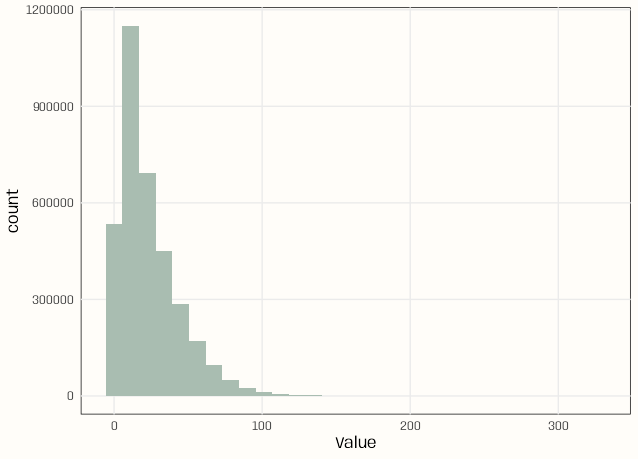
notebook_colors <- unname(swatches::read_ase(here::here("palettes/Forest Floor.ase"))) ds_no2_clean |> select(Value) |> filter(!is.nan(Value)) |> collect() |> ggplot(aes(x = Value)) + geom_histogram(fill = notebook_colors[[2]]) + theme_notebook()- I’m using ds_no2_clean instead of ds_no2_raw. See for details on the cleaning
- The x-axis is fine. As seen in the
skim_arrowresults, the max value is 326
Tables
ds_no2_clean |> count(location, sort = TRUE) |> collect() |> pull(n) |> table() #> 8759 #> 412- All 412 locations have the same number of observations
- location was formerly Samplingpoint but I extracted the main location code part of the string.
Partitioning
Partitioning increases the number of files and it creates a directory structure around the files.
Hive Partitioning - Folder/file structure based on partition keys (i.e. grouping variable). Within each folder, the key has a value determined by the name of the folder. By partitioning the data in this way, it makes it faster to do queries on data slices.
Example: Folder structure when partitioning on year and month
taxi-data
   year=2018
     month=01
      file01.parquet
     month=02
      file02.parquet
      file03.parquet
     ...
   year=2019
     month=01
     ...
Pros
- Allows Arrow to construct a more efficient query
- Can be read and written with parallelism
Cons
- Each additional file adds a little overhead in processing for filesystem interaction
- Can increase the overall dataset size since each file has some shared metadata
Best Practices
View metadata of a partitioned dataset
air_data <- open_dataset("airquality_partitioned_deeper") # View data air_data ## FileSystemDataset with 153 Parquet files ## Ozone: int32 ## Solar.R: int32 ## Wind: double ## Temp: int32 ## Month: int32 ## Day: int32 ## ## See $metadata for additional Schema metadata- This is a “dataset” type so data won’t be read into memory
- Assume
$metadatawill indicate which columns the dataset is partitioned by
Partition a large file and write to arrow format
lrg_file <- open_dataset(<file_path>, format = "csv") lrg_file %>% group_by(var) %>% write_dataset(<output_dir>, format = "feather")- Pass the file path to
open_dataset() - Use
group_by()to partition the Dataset into manageable chunks- Can also use partitioning in
write_dataset
- Can also use partitioning in
- Use
write_dataset()to write each chunk to a separate Parquet file—all without needing to read the full CSV file into R open_datasetis fast because it only reads the metadata of the file system to determine how it can construct queries
- Pass the file path to
Partition Columns
Preferrably chosen based on how you expect to use the data (e.g. important group variables)
Example: partition on county because your analysis or transformations will largely be done by county even though since some counties may be much larger than others and will cause the partitions to be substantially imbalanced.
If there is no obvious column, partitioning can be dictated by a maximum number of rows per partition
write_dataset( data, format = "parquet", path = "~/datasets/my-data/", max_rows_per_file = 1e7 ) dat <- open_dataset("~/datasets/my-data")- Files can get very large without a row count cap, leading to out-of-memory errors in downstream readers.
- Relationship between row count and file size depends on the dataset schema and how well compressed (if at all) the data is
- Other ways to control file size.
- “max_rows_per_group” - splits up large incoming batches into multiple row groups.
- If this value is set then “min_rows_per_group” should also be set or else you may end up with very small row groups (e.g. if the incoming row group size is just barely larger than this value).
- “max_rows_per_group” - splits up large incoming batches into multiple row groups.
Fixed Precision Decimal Numbers
Computers don’t store exact representations of numbers, so there are floating point errors in calculations. Doesn’t usually matter in analysis, but it can matter in transaction-based operations.
txns <- tibble(amount = c(0.1, 0.1, 0.1, -0.3)) %>%
    summarize(balance = sum(amount, na.rm = TRUE
# Should be 0
txns
# 5.55e-17
The accumulation of these errors can be costly.
Arrow can fix this with fixed precision decimals
# arrow table (c++ library)
# collect() changes it to a df
txns <- Table$create(amount = c(0.1, 0.1, 0.1, -0.3))
txns$amount <- txns$amount$cast(decimal(3,2))
txns
# blah, blah, decimal128, blah

write_parquet(txns, "data/txns_decimal.parquet")
txns <- spark_read_parquet("data/txns_decimal.parquet")
txns %>%
    summarize(balance = sum(ammount, na.rm = T))
# balance
#    0
Queries
Example: Filter partitioned files
library(dbplyr) # iris dataset was written and partitioned to a directory path stored in dir_out ds <- arrow::open_dataset(dir_out, partitioning = "species") # query the dataset ds %>% filter(species == "species=setosa") %>% count(sepal_length) %>% collect()- Format: “<partition_variable>=<partition_value>”
computestores the result in Arrowcollectbrings the result into R
Example: libarrow functions
arrowmagicks %>% mutate(days = arrow_days_between(start_date, air_date)) %>% collect()- “days_between” is a function in libarrow but not in {arrow}. In order to use it, you only have to put the “arrow_” prefix in front of it.
- Use
list_compute_functionsto get a list of the available functions- List of potential functions available (libarrow function reference)
When the query is also larger than memory
library(arrow) library(dplyr) nyc_taxi <- open_dataset("nyc-taxi/") nyc_taxi |> filter(payment_type == "Credit card") |> group_by(year, month) |> write_dataset("nyc-taxi-credit")- In the example, the input is 1.7 billion rows (70GB), output is 500 million (15GB). Takes 3-4 mins.
- See Operations >> Example: Foursquare Sample. This seems like it would blow up your RAM. But, maybe it’s the current version of the package that I have, and its a bug.
User-defined functions
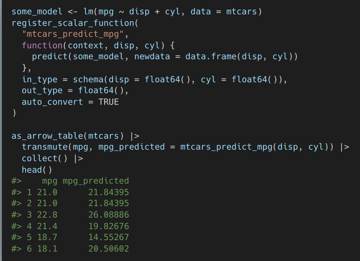
register_scalar_function- accepts base R functions inside your function
Example: Collect Then Wrangle List Column
library(arrow) library(dplyr) library(dbplyr) arr_fsq <- open_dataset("~/R/Data/foursquare-spaces/") tib_comp_fsq <- arr_fsq |> select(name, fsq_category_labels, locality, region, address, latitude, longitude, geom, bbox) |> filter(locality == 'Louisville' & region == 'KY') |> collect() |> tidyr::unnest_auto(fsq_category_labels) |> filter(stringr::str_detect(fsq_category_labels, "Car Dealership")) |> distinct(name, .keep_all = TRUE)- For other methods of performing this query, see
- Databases. DuckDB >> dbplyr >> Example 1
- Databases, DuckDB >> SQL >> Example 1, Example 2
- This method was a little memory intensive. it’s querying 10 GB of parquet files, and it raised my RAM usage by around 900 MB.
- For other methods of performing this query, see
DuckDB
Converting a csv to parquet
SET threads = 4 ;
COPY 'data_recensement_2017.csv' TO 'data_recensement_2017.parquet'
(compression zstd) ;
threads is set to the number of threads available by default
Will automatically detect the type of delimiter
Query
df <- duckdb:::sql("FROM 'file.parquet'")Export a DuckDB database to parquet
drv <- duckdb::duckdb()
con <- DBI::dbConnect(drv)
on.exit(DBI::dbDisconnect(con), add = TRUE)

# create duckdb table
DBI::dbWriteTable(con, "mtcars", mtcars)

DBI::dbExecute(con, DBI::sqlInterpolate(con,
  "COPY mtcars TO ?filename (FORMAT 'parquet', COMPRESSION 'snappy')",
  filename = 'mtcars.parquet'
))
Cloud
Access files in Amazon S3 (works for all file types)
taxi_s3 <- read_parquet("s3://ursa-labs-taxi-data/2013/12/data.parquet)
# multiple files
ds_s3 <- open_dataset(s3://ursa-labs-taxi-data/", partitioning = c("year", "month"))
As of 2021, only works for Amazon uri
read_parquetcan take a minute to loadYou can see the folder structure in the read_parquet S3 uri
Example Query
# over 125 files and 30GB ds_s3 %>% filter(total_amount > 100, year == 2015) %>% select(tip_amount, total_amount, passenger_count) %>% mutate(tip_pct = 100 * tip_amount / total_amount) %>% group_by(passenger_count) %>% summarize(median_tip_pct = median(tip_pct), n = n()) %>% print() # is this necessary?- Partitioning allowed Arrow to bypass all files that weren’t in year 2015 directory and only perform calculation on those files therein.
Access Google Cloud Storage (GCS)
Geospatial
Also see Databases, DuckDB >> Geospatial
Packages
- {geoarrow} - Leverages the features of the arrow package and larger Apache Arrow ecosystem for geospatial data
- {lazysf} (README has better documentation)- Provides a {dplyr} backend for any vector data source (aka shapefiles) readable by GDAL (e.g. gpkg, shp, geojson).
- Uses
gdalraster::GDALVectorto talk to GDAL and {dbplyr} for SQL translation, giving you lazy evaluation of spatial data through familiar {dplyr} verbs. - For larger datasets, enable GDAL’s columnar Arrow C stream interface through nanoarrow for faster data transfer (link)
- Uses
Resources
Types
- GEOMETRY type represents planar spatial objects. This includes points, linestrings, polygons, and multi geometries. The logical type indicates that the column contains spatial objects, while the physical storage uses a standard binary encoding.
- The GEOGRAPHY type is similar to GEOMETRY but represents objects on a spherical or ellipsoidal Earth model. Geography values are encoded using longitude and latitude coordinates expressed in degrees.
Example: (source)
import geoarrow.pyarrow as ga # For GeoArrow extension type registration
import geopandas
import pyarrow as pa
from pyarrow import parquet

# From GeoPandas, create a GeoDataFrame from your favourite data source
url = "https://raw.githubusercontent.com/geoarrow/geoarrow-data/v0.2.0/natural-earth/files/natural-earth_countries.fgb"
df = geopandas.read_file(url)

# Write to Parquet using pyarrow.parquet()
tab = pa.table(df.to_arrow())
parquet.write_table(tab, "countries.parquet")

# Verify that the Geometry logical type was written to the file
parquet.ParquetFile("countries.parquet").schema
#> <pyarrow._parquet.ParquetSchema object at 0x10776dac0>
#> required group field_id=-1 schema {
#>   optional binary field_id=-1 name (String);
#>   optional binary field_id=-1 continent (String);
#>   optional binary field_id=-1 geometry (Geometry(crs=));
#> }

# Geometry is read to a pyarrow.Table as GeoArrow arrays that can be
# converted back to GeoPandas
tab = parquet.read_table("countries.parquet")
df = geopandas.GeoDataFrame.from_arrow(tab)
df.head(2)
#> name continent  \
#> 0                         Fiji   Oceania
#> 1  United Republic of Tanzania    Africa
#>
#>                                             geometry
#> 0  MULTIPOLYGON (((180 -16.06713, 180 -16.55522, ...
#> 1  MULTIPOLYGON (((33.90371 -0.95, 34.07262 -1.05...