Priors
Misc
- Packages
- {makemyprior} (paper)- Intuitive construction of Joint priors for variance parameters.
- GUI can be used to choose the joint prior, where the user can click through the model and select priors.
- Using a hierarchical variance decomposition, a joint variance prior is formulated that takes the whole model structure into account. In this way, existing knowledge can intuitively be incorporated at the level it applies to.
- Alternatively, independent variance priors can be used for each model component in the latent Gaussian model.
- {makemyprior} (paper)- Intuitive construction of Joint priors for variance parameters.
- Resources
- Stan/brms prior distributions
- Distributions are towards the bottom of the guide
- {brms} should have all the distributions available in Stan according to their docs (see Details section)
- Prior Distributions for rstanarm Models
- Slides: Weakly Informative Priors (Gelman)
- Prior Choice Recommendations (Vehtari)
- Stan/brms prior distributions
- Papers
- Using meta-analyis or previous studies to create informed priors
- “Systematic use of informed studies leads to more precise, but more biased estimates (due to non-linear information flow in the literature). Critical comparison of informed and skeptical priors can provide more nuanced and solid understanding of our findings.” (thread + paper)
- i.e. try both and compare the result
- “Systematic use of informed studies leads to more precise, but more biased estimates (due to non-linear information flow in the literature). Critical comparison of informed and skeptical priors can provide more nuanced and solid understanding of our findings.” (thread + paper)
- Prior sensitivity analysis
- {priorsense}
Example: (source)
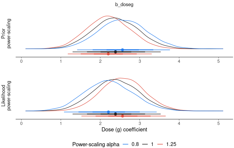
brms_fit |>
  powerscale_plot_dens(variable = 'b_doseg', help_text = FALSE) +
  labs(x = 'Dose (g) coefficient', y = NULL)

powerscale_sensitivity(brms_fit, variable = 'b_doseg')
#>  Sensitivity based on cjs_dist:
#>  variable prior likelihood diagnosis
#>  b_doseg  0.236      0.219 prior-data conflict
- {BayesSenMC}
- For binary exposure and a dichotomous outcome
- Generates different posterior distributions of adjusted odds ratio under different priors of sensitivity and specificity, and plots the models for comparison. It also provides estimations for the specifications of the models using diagnostics of exposure status with a non-linear mixed effects model.
- Vignette
- {priorsense}
- Shrinkage and Regularization (source)
- Also see R2D2 and Horseshoe papers in Papers section
- Unlike non-Bayesian counterparts such as the lasso, shrinkage priors also provide adequate uncertainty quantification for parameters of interest
- The spike-and-slab prior become intractable for even a moderate number of predictors
- The global–local class of prior distributions is a popular and successful mechanism for providing shrinkage and regularization
- Use continuous scale mixtures of Gaussian distributions to produce desirable shrinkage properties, such as (approximate) sparsity or smoothness
- Global–Local priors that shrink towards sparsity, such as the horseshoe prior, produce competitive estimators with greater scalability and are validated by theoretical results, simulation studies and a variety of applications.
- Statistical Rethinking
- The “flatness” of a Normal prior is controlled by the size of the s.d. value
- not in logistic regression (see examples below)
- Flat priors result in poor frequency properties (i.e. consistently give bad inferences) in realistic settings where studies are noisy and effect sizes are small. (Gelman post)
- Weakly informative priors: they allow some implausibly strong relationships but generally bound the lines to possible ranges of the variables. (fig 5.3, pg 131)
- We want our priors to be skeptical of large differences [in treatment effects], so that we reduce overfitting. Good priors hurt fit to sample but are expected to improve prediction. (pg 337)
- We don’t formulate priors based on the sample data. We want the prior predictive distribution to live in the plausible outcome space, not fit the sample.
- For logistic regression and poisson regression, a flat prior in the logit space is not a flat prior in the outcome probability space (pg 336)
- As long as the priors are vague, minimizing the sum of squared deviations to the regression line is equivalent to finding the posterior mean. pg 200
- “As always in rescaling variables, the goals are to create focal points that you might have prior information about, prior to seeing the actual data values. That way we can assign priors that are not obviously crazy, and in thinking about those priors, we might realize that the model makes no sense. But this is only possible if we think about the relationship between measurements and parameters, and the exercise of rescaling and assigning sensible priors helps us along that path. Even when there are enough data that choice of priors is not crucial, this thought exercise is useful.” pg 258
- Comparing the posteriors with the priors
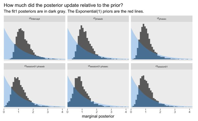
- The “flatness” of a Normal prior is controlled by the size of the s.d. value
Preprocessing
- Centering the predictor
- Makes the posterior easier to sample
- Reduces covariance among the parameter posterior distributions
- Makes it easier to define the prior on average temperature in the center of the time range (instead defining prior for temperature at year 0).
- Links to Gelman posts about centering your predictors (article)
- If you standardize your predictors, you can use a mean of 0 for the prior on your intercept
- With flat priors, this doesn’t make much of difference
Get Prior Recommendations
Example: Fitting a spline
# get recommended prior specifications # s is the basis function brms imports from mgcv pkg brms::get_prior(data = d2, family = gaussian, doy ~ 1 + s(year)) ## prior class coef group resp dpar nlpar bound source ## (flat) b default ## (flat) b syear_1 (vectorized) ## student_t(3, 105, 5.9) Intercept default ## student_t(3, 0, 5.9) sds default ## student_t(3, 0, 5.9) sds s(year) (vectorized) ## student_t(3, 0, 5.9) sigma default # applying the recommendations # multi-level method for spline fitting b4.11 <- brm(data = d2, family = gaussian, # k = 19, corresponds to 17 basis functions I guess ::shrugs:: # The default for s() is to use what’s called a thin plate regression spline # bs uses a basis spline temp ~ 1 + s(year, bs = "bs", k = 19), prior = c(prior(normal(100, 10), class = Intercept), prior(normal(0, 10), class = b), prior(student_t(3, 0, 5.9), class = sds), prior(exponential(1), class = sigma)), iter = 2000, warmup = 1000, chains = 4, cores = 4, seed = 4, control = list(adapt_delta = .99))Example: Multinomial Logistic Regression
# Outcome categorical variable has k = 3 levels. We fit k-1 models. Hence the 2 intercept priors # intercept model get_prior(data = d, # refcat sets the reference category to the 3rd level family = categorical(link = logit, refcat = 3), # just an intercept model career ~ 1) ## prior class coef group resp dpar nlpar bound source ## (flat) Intercept default ## student_t(3, 3, 2.5) Intercept mu1 default ## student_t(3, 3, 2.5) Intercept mu2 default b11.13io <- brm(data = d, family = categorical(link = logit, refcat = 3), career ~ 1, prior = c(prior(normal(0, 1), class = Intercept, dpar = mu1), prior(normal(0, 1), class = Intercept, dpar = mu2)), iter = 2000, warmup = 1000, cores = 4, chains = 4, seed = 11, file = "fits/b11.13io")- As of brms 2.12.0, “specifying global priors for regression coefficients in categorical models is deprecated.” Meaning — if we want to use the same prior for both, we need to use the
dparargument for each
- As of brms 2.12.0, “specifying global priors for regression coefficients in categorical models is deprecated.” Meaning — if we want to use the same prior for both, we need to use the
Formulating an Intercept Prior
Example SR 6.3.1 pgs 182-83
- A thought process on how to set a predictor prior based on its relationship to the outcome and an intercept prior.
Example SR 7.1.1 pg 200
- Outcome variable was scaled, outcome/max(outcome)
- Values now between 0 and 1
- Useful for when 0 is a meaningful boundary
- Now able to center the intercept prior on mean of outcome, α ∼ Normal(0.5, 1)
- Says that the average species with an average body mass (predictor variable) has a brain volume (outcome variable) with an 89% credible interval (± 1.5 sd) from about −1 to 2.
- Body mass was centered, so it’s at its average is when its value is zero.
- Says that the average species with an average body mass (predictor variable) has a brain volume (outcome variable) with an 89% credible interval (± 1.5 sd) from about −1 to 2.
- Outcome variable was scaled, outcome/max(outcome)
Example SR 8.3.2 pg 259
Similar to 7.1.1 example except there’s the observation that a sd = 1 for the intercept prior is too large given that the outcome is bdd between 0 and 1 (after scaling)
a <- rnorm( 1e4 , 0.5 , 1 ) sum( a < 0 | a > 1 ) / length( a ) [1] 0.6126- 61% of the prior is outside the bounds for the outcome which makes no sense
If it’s 0.5 units from the mean to zero, then a standard deviation of 0.25 should put only 5% of the mass outside the valid range.
a <- rnorm( 1e4 , 0.5 , 0.25 ) sum( a < 0 | a > 1 ) / length( a ) [1] 0.0486- Not sure why you want 5% outside the valid range of the outcome variable
Example (Ch 11 pg 335-6)
With logistic regression, flat Normal priors aren’t priors with a high sd.
.png)
- The Normal prior on the logit scale with the large sd says that the probabilty of an event is either 0 or 1 which usually isn’t reasonable.
- logit(pi) = α
- α ~ Normal(0, 1.5) — the curve for the probability of an event is very flat, looks like a mesa
- α ~ Normal(0, 1.0) —the curve for the probability of an event is a fat hill shape. A little more skeptical of extreme probabilities
- The Normal prior on the logit scale with the large sd says that the probabilty of an event is either 0 or 1 which usually isn’t reasonable.
Example
Also have ggplot code in Documents >> R >> Code >> Simulations >> sim-prior-predictive-distr.R
Poisson regression (pg 356)
In poisson regression, flat normal priors aren’t priors with high s.d.
.png)
# prior predictive distribution
curve( dlnorm( x , 3 , 0.5 ) , from=0 , to=100 , n=200 )
Since poisson regression uses a log link, the outcome is log-normal. We’re simulating the effect of a normal prior on a log-normal outcome which is why the simulation code uses
dlnorm.“number of tools” is the outcome variable
The prior with s.d. 10 has almost all the probability density at zero and huge mean
a <- rnorm(1e4,0,10)
lambda <- exp(a)
mean(lambda)
[1] 9.622994e+12
This usually doesn’t make sense for a prior
The prior with s.d. 0.5 has a mean around 20 and a more spread out probability density which makes much more sense given the literature on the subject.
Formulating a Slope Prior
Example SR pg 259
- slopes centered on zero, imply no prior information about direction
- How big could can the slopes be in theory?
- After centering, range of each predictor is 2—from −1 to 1 is 2 units.
- To take us from the theoretical minimum of outcome variable = 0 on one end to the observed maximum of 1—a range of 1 unit—on the other would require a slope of 0.5 from either predictor variable—0.5 × 2 = 1.
- Assign a standard deviation of 0.25, then 95% of the prior slopes are from −0.5 to 0.5, so either predictor could in principle account for the entire range, but it would be unlikely
Example SR pg 336-7
- With logistic regression, flat Normal priors aren’t priors with a high sd.
.png)
- Shows difference between two levels of the treatment effect (i.e. 2 different treatments) on the 0/1 outcome
- The prior with large sd has all the probability density massed at 0 and 1
- Says that the 2 treatments are completely alike or completely different
- The prior with the small sd (e.g. Normal(0, 0.5) is concentrated from about 0 to about 0.4
- Although 0 difference in treatments has the highest probability, the mean is at a difference around 0.10
- Prior says that large differences between treatments are very unlikely, but if the data contains strong evidence of large differences, they will shine through
- Pairs nicely with an intercept prior, α ~ Normal(0, 1.5)
- An example of a weakly informative prior that reduces overfitting the sample data
- Although 0 difference in treatments has the highest probability, the mean is at a difference around 0.10
- With logistic regression, flat Normal priors aren’t priors with a high sd.
Example: pg 357
.png)
set.seed(11) ## TOP ROW # how many lines would you like? n <- 100 # simulate and wrangle tibble(i = 1:n, a = rnorm(n, mean = 3, sd = 0.5)) %>% mutate(`beta%~%Normal(0*', '*10)` = rnorm(n, mean = 0 , sd = 10), `beta%~%Normal(0*', '*0.2)` = rnorm(n, mean = 0 , sd = 0.2)) %>% pivot_longer(contains("beta"), values_to = "b", names_to = "prior") %>% expand(nesting(i, a, b, prior), x = seq(from = -2, to = 2, length.out = 100)) %>% # plot ggplot(aes(x = x, y = exp(a + b * x), group = i)) + geom_line(size = 1/4, alpha = 2/3, color = wes_palette("Moonrise2")[4]) + labs(x = "log population (std)", y = "total tools") + coord_cartesian(ylim = c(0, 100)) + facet_wrap(~ prior, labeller = label_parsed) ## BOTTOM ROW prior <- tibble(i = 1:n, a = rnorm(n, mean = 3, sd = 0.5), b = rnorm(n, mean = 0, sd = 0.2)) %>% expand(nesting(i, a, b), x = seq(from = log(100), to = log(200000), length.out = 100)) # left p1 <- prior %>% ggplot(aes(x = x, y = exp(a + b * x), group = i)) + geom_line(size = 1/4, alpha = 2/3, color = wes_palette("Moonrise2")[4]) + labs(subtitle = expression(beta%~%Normal(0*', '*0.2)), x = "log population", y = "total tools") + coord_cartesian(xlim = c(log(100), log(200000)), ylim = c(0, 500)) # right p2 <- prior %>% ggplot(aes(x = exp(x), y = exp(a + b * x), group = i)) + geom_line(size = 1/4, alpha = 2/3, color = wes_palette("Moonrise2")[4]) + labs(subtitle = expression(beta%~%Normal(0*', '*0.2)), x = "population", y = "total tools") + coord_cartesian(xlim = c(100, 200000), ylim = c(0, 500)) # combine p1 | p2- With poisson regression, flat Normal priors aren’t priors with a high sd.
- Outcome: total_tools, predictor: log_population
- Bottom row fig titles have a typo. Should be a ~ dnorm(3, 0.5) since it’s the Intercept prior
- Variables have been standardized; total_tools simulated with intercept + predictor priors. So the y axis is simulating the potential fitted values.
- Top Left (0 is mean of log_population):
- large sd: mostly results in explosive growth of tools just after mean of log_population or explosive decline just before mean log_population (unlikely)
- Top Right (0 is mean of log_population)
- small sd (flatter): most results are around the mean of the intercept prior results (see above) but still allows for more extreme estimates. (reasonable)
- Bottom Left
- 100 trend lines between total tools and un-standardized log population
- Viewing prior predictive trends with un-standardized variables is more natural to see what’s happening
- 100 total tools is probably the most we expect to ever see in these data
- Looks like 80-85% of the trend lines are under 100. still keeps some explosive possibilities.
- 100 trend lines between total tools and un-standardized log population
- Bottom Right
- 100 trend lines between total tools and un-standardized, un-logged population
- Viewing prior predictive trends with un-standardized, un-transformed variables is even more natural to see what’s happening
- When a predictor variable is logged in a regression with a log-link (i.e. log-log), this means we are assuming diminishing returns for the raw predictor variable.
- Each additional person contributes a smaller increase in the expected number of tools
- Diminishing returns as a predictor value continues to increase makes sense in many situations which is why logging predictors is a popular transformation
- 100 trend lines between total tools and un-standardized, un-logged population
- Thoughts
- Bottom-right seems like the right way to visualize the prior to think about the association between the outcome and predictor
- Top row and bottom-left seem to give a better sense of how many explosive possibilities and their patterns that your allowing for with different transformations
Formulating a Sigma Prior
- Common to start with
exponential(1) - Tightening the spread of the Exponential distribution by using a Gamma distribution (Thread)
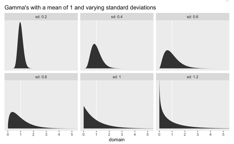
- You can keep “mean = 1” (aka exponential(1) and adjust the “sd”.
- See Distributions >> Gamma for details on the process
- Also allows you to move most of the mass of the prior a littler further away from 0.
- Another alternative is the Weibull distribution
- You can keep “mean = 1” (aka exponential(1) and adjust the “sd”.
- Random Effects
- For a GLMM logistic regression, to get a flat sigma prior (on the probability scale) for the random effects, see article, thread
- The last part of the article where he goes through a “grid search” is confusing to me, so I’ll need to run the code to figure out what he’s doing
- T.J. Mahr is in the thread with a convenient helper function from a package, but again I need to understand the end of the article to understand how his tip fits.
- For a GLMM logistic regression, to get a flat sigma prior (on the probability scale) for the random effects, see article, thread
- Logistic Regression
Using the relationship between log odds and Cohen’s d
\[\sigma_{\text{log odds}} = d \times \frac{\pi}{\sqrt{3}}\]
\(d\) is hypothesized effect size given by Cohen’s d
Notes from
Guidelines
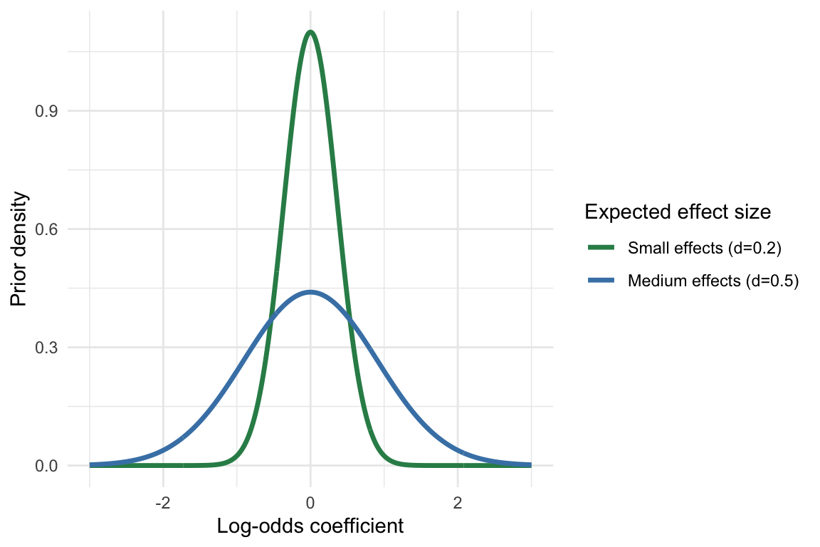
- Small effect: d ≈ 0.2
- Medium effect: d ≈ 0.5
- Large effect: d ≈ 0.8
\(\sigma_{\text{log odds}}\) will be the sigma parameter for your Normal prior
Example: Small-Medium Size Effect
d_expected <- 0.3
prior_sd <- d_expected * pi / sqrt(3)  # ≈ 0.54

# Define priors for all coefficients
priors <- c(
  prior(normal(0, prior_sd), class = b)  # All slopes get the same prior
)
Extracting a Prior From a Model
- Example: Logistic Regression (SR sect 11.1.1 pg 336)
Intercept
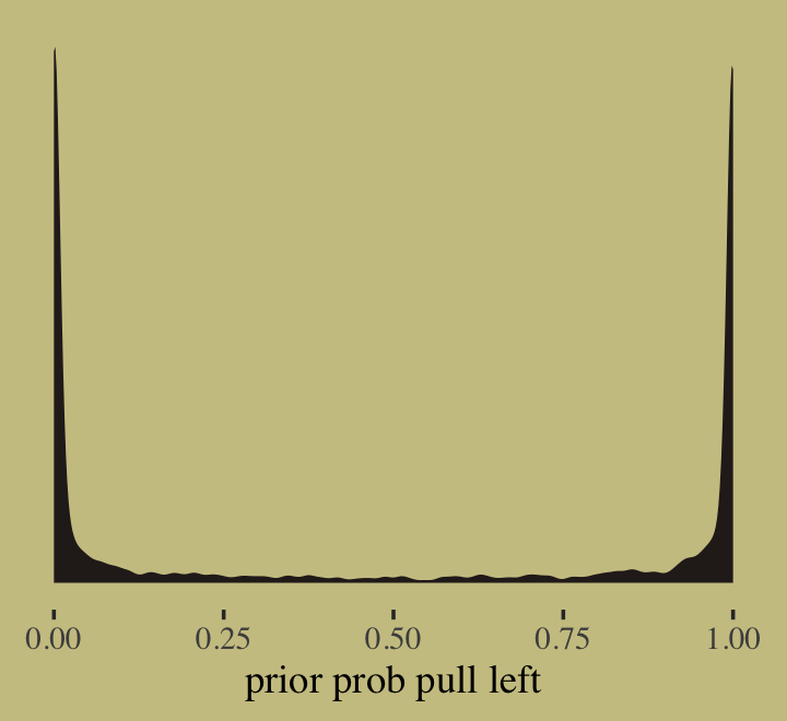
# prior_samples and inv_logit_scaled are brms functions
# theme is from ggthemes
prior_samples(b11.1) %>%
  mutate(p = inv_logit_scaled(Intercept)) %>%

  ggplot(aes(x = p)) +
  geom_density(fill = wes_palette("Moonrise2")[4],
               size = 0, adjust = 0.1) +
  scale_y_continuous(NULL, breaks = NULL) +
  xlab("prior prob pull left")
Simulating a Prior Predictive Distribution
Notes from Visualization in Bayesian Workflow
If we specify proper priors for all parameters in the model, a Bayesian model yields a joint prior distribution on parameters and data, and hence a prior marginal distribution for the data, i.e. Bayesian models with proper priors are generative models.
- We cannot fully understand the prior by fixing all except one parameter and assessing the effect of the unidimensional marginal prior. Instead, we need to assess the effect of the prior as a multivariate distribution.
The main advantage to assessing priors based on the prior marginal distribution for the data is that it reflects the interplay between the prior distribution on the parameters and the likelihood. This is a vital component of understanding how prior distributions actually work for a given problem
It is important that this prior predictive distribution for the data has at least some mass around extreme but plausible data sets. However, there should be no mass on completely implausible data sets.
{performance::check_priors} takes a fitted model (stan, brms, rstanarm) and the name of a predictor.
Example:
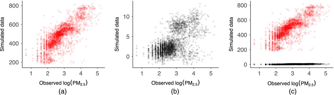
- Left: Shows data generated from “vague” priors. The Y-Axix is shows the generated data from these priors are completely outside the range of possible PM 2.5 values
- Center: Shows a data generated from weakly informative priors which are plausible.
- Right: Showing both on the same chart which emphasizes how the exteme the difference is between the generated data.
Example: SR pg 176
# log-normal prior
sim_p <- rlnorm(1e4 , 0 , 0.25)

# "this prior expects anything from 40% shrinkage up to 50% growth"
rethinking::precis( data.frame(sim_p) )
# 'data.frame': 10000 obs. of 1 variables:
#       mean    sd  5.5% 94.5% histogram
# sim_p 1.03  0.26  0.67  1.48 ▁▃▇▇▃▁▁▁▁▁▁

# tidy-way
sim_p <-
  tibble(sim_p = rlnorm(1e4, meanlog = 0, sdlog = 0.25)) %>%
    mutate(`exp(sim_p)` = exp(sim_p)) %>%
    gather() %>%
    group_by(key) %>%
    tidybayes::mean_qi(.width = .89) %>%
    mutate_if(is.double, round, digits = 2)

## # A tibble: 2 x 7
##  key         value .lower .upper .width .point .interval
##  <chr>       <dbl>  <dbl>  <dbl>  <dbl>  <chr>     <chr>
## 1 exp(sim_p)  2.92   1.96   4.49   0.89   mean        qi
## 2 sim_p       1.03   0.67    1.5   0.89   mean        qi
Visualize with ggplot
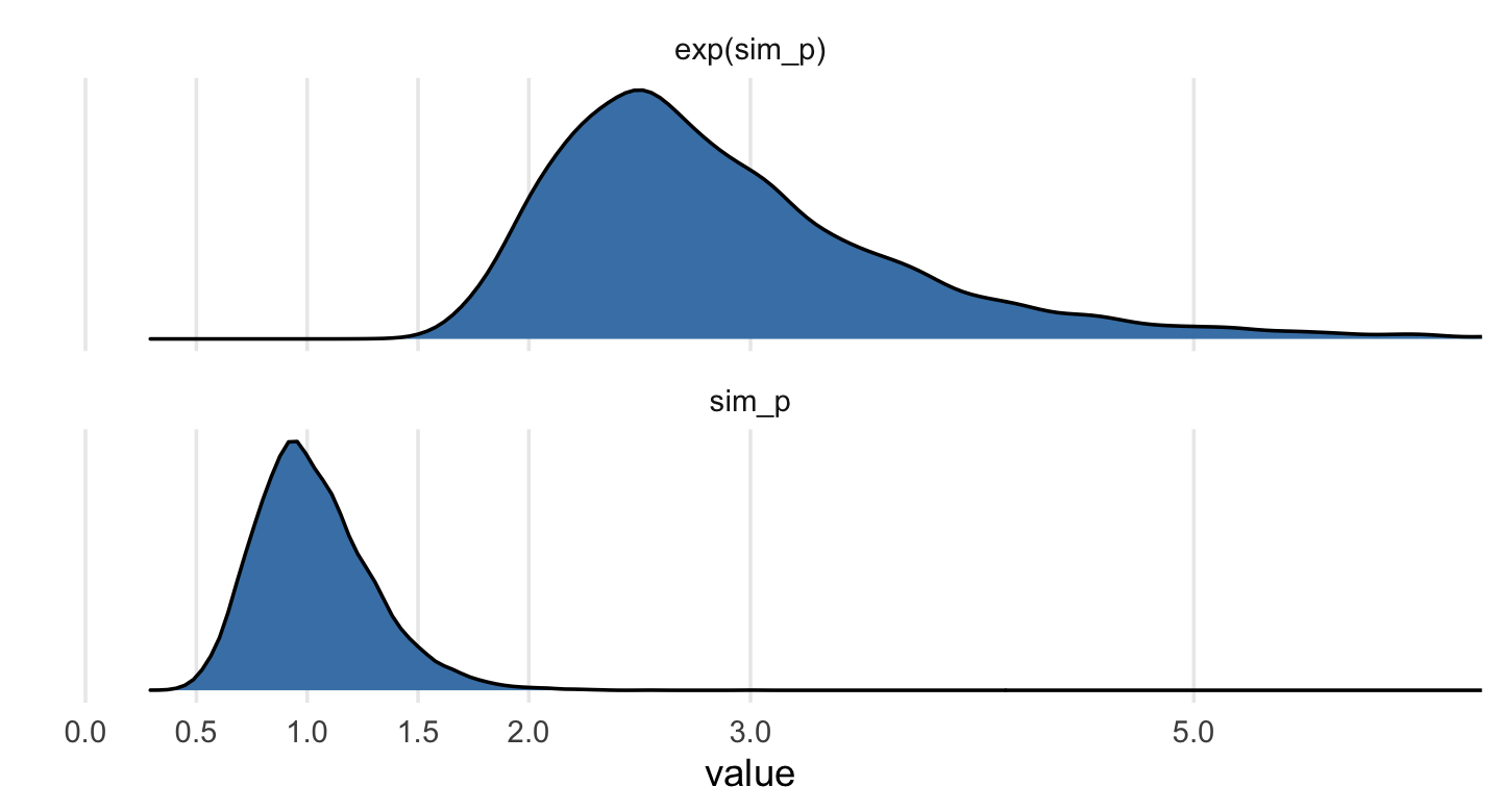
# wrangle
sim_p %>%
  mutate(`exp(sim_p)` = exp(sim_p)) %>%
  gather() %>%
  # plot
  ggplot(aes(x = value)) +
  geom_density(fill = "steelblue") +
  scale_x_continuous(breaks = c(0, .5, 1, 1.5, 2, 3, 5)) +
  scale_y_continuous(NULL, breaks = NULL) +
  coord_cartesian(xlim = c(0, 6)) +
  theme(panel.grid.minor.x = element_blank()) +
  facet_wrap(~key, scale = "free_y", ncol = 1)
Example:
Possible Intercept Priors
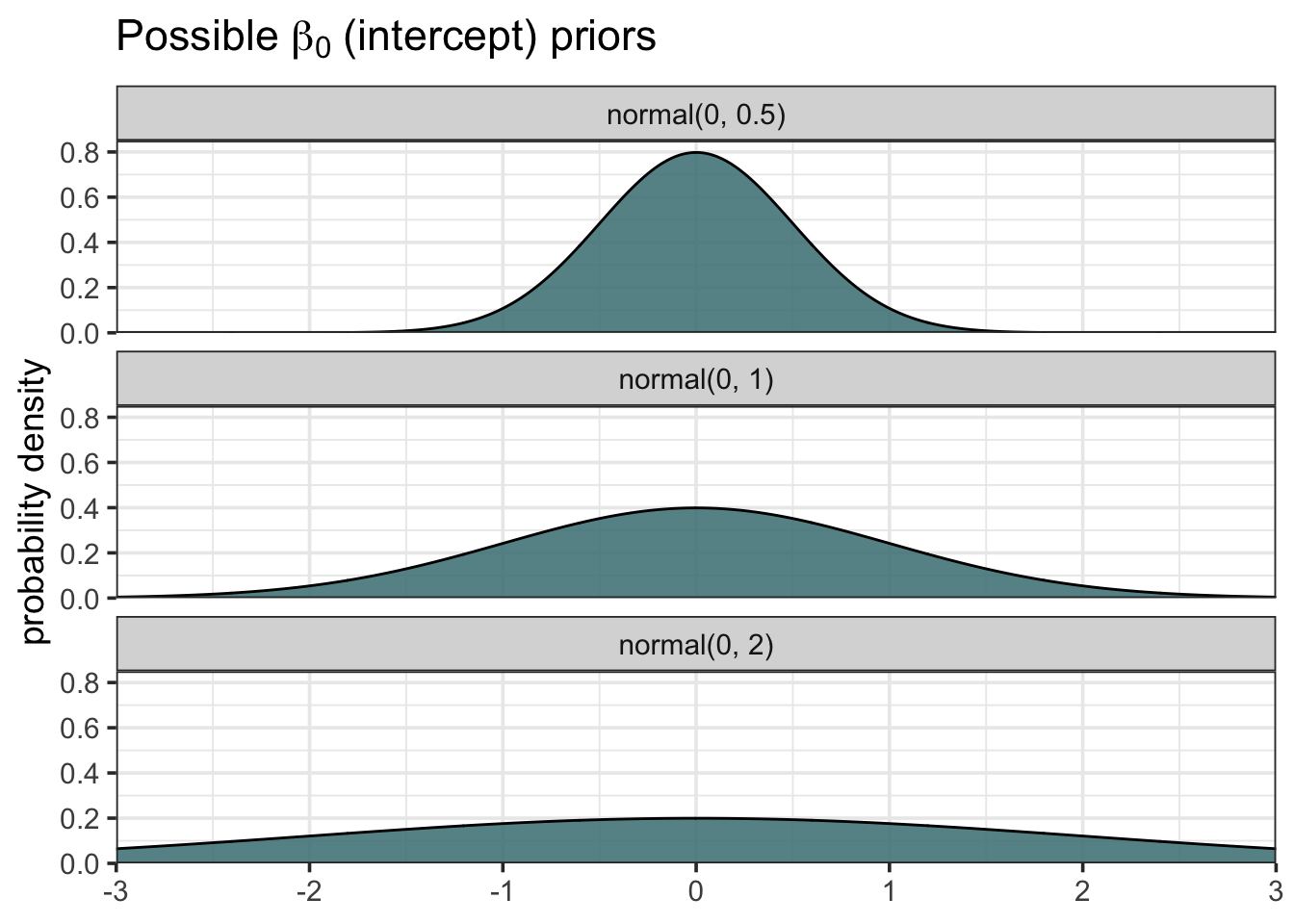
grid <- seq(-3, 3,
             length.out = 1000) # evenly spaced values from -3 to 3
b0_prior <-
   map_dfr(.x = c(0.5, 1, 2), # .x represents the three sigmas
           ~ data.frame(grid = grid,
                        b0 = dnorm(grid, mean = 0, sd = .x)),
                        .id = "sigma_id")
# Create Friendlier Labels
b0_prior <- b0_prior %>%
  mutate(sigma_id = factor(sigma_id,
         labels = c("normal(0, 0.5)",
                    "normal(0, 1)",
                    "normal(0, 2)")))
ggplot(b0_prior, aes(x = grid, y = b0)) +
  geom_area(fill = "cadetblue4", color = "black", alpha = 0.90) +
  scale_x_continuous(expand = c(0, 0)) +
  scale_y_continuous(expand = c(0, 0), limits = c(0, 0.85)) +
  labs(x = NULL,
       y = "probability density",
       title = latex2exp::TeX("Possible $\\beta_0$ (intercept) priors")) +
       facet_wrap(~sigma_id, nrow = 3)
Sampling of lines from \(\beta_0\) and \(\beta_1\) priors
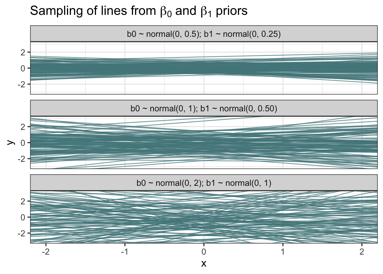
b0b1 <-
  map2_df(.x = c(0.5, 1, 2),
          .y = c(0.25, 0.5, 1),
          ~ data.frame(
              b0 = rnorm(100, mean = 0, sd = .x),
              b1 = rnorm(100, mean = 0, sd = .y)),
          .id = "sigma_id"
  )

# Create friendlier labels
b0b1 <-
  b0b1 %>%
    mutate(sigma_id = factor(sigma_id,
                             labels = c("b0 ~ normal(0, 0.5); b1 ~ normal(0, 0.25)",
                                        "b0 ~ normal(0, 1); b1 ~ normal(0, 0.50)",
                                        "b0 ~ normal(0, 2); b1 ~ normal(0, 1)")))

ggplot(b0b1) +
  geom_abline(aes(intercept = b0, slope = b1), color = "cadetblue4", alpha = 0.75) +
  scale_x_continuous(limits = c(-2, 2)) +
  scale_y_continuous(limits = c(-3, 3)) +
  labs(x = "x",
       y = "y",
  title = latex2exp::TeX("Sampling of lines from $\\beta_0$ and $\\beta_1$ priors")) +
  facet_wrap(~sigma_id, nrow = 3)
Conjugate Priors
If the posterior distributions p(θ | x) are in the same probability distribution family as the prior probability distribution p(θ), the prior and posterior are then called conjugate distributions, and the prior is called a conjugate prior for the likelihood function p(x | θ)
Benefits
- Bayesian updates no longer need to compute the product of the likelihood and prior (only addition is needed).
- This product is computationally expensive and sometimes not feasible.
- Otherwise numerical integration may be necessary
- May give intuition, by more transparently showing how a likelihood function updates a prior distribution.
- Bayesian updates no longer need to compute the product of the likelihood and prior (only addition is needed).
All members of the exponential family have conjugate priors.
List
<Beta posterior>
Beta prior * Bernoulli likelihood → Beta posterior
Beta prior * Binomial likelihood → Beta posterior
Beta prior * Negative Binomial likelihood → Beta posterior
Beta prior * Geometric likelihood → Beta posterior

<Gamma posterior>
Gamma prior * Poisson likelihood → Gamma posterior
Gamma prior * Exponential likelihood → Gamma posterior

<Normal posterior>
Normal prior * Normal likelihood (mean) → Normal posterior

<Others>
Dirichlet prior * Multinomial likelihood → Dirichlet posterior
Prior Elicitation
- Translating expert opinion to a probability density than you can use as a prior
- Misc
- Notes from:
- Video: On using expert information in Bayesian statistics (R >> Videos)
- Paper: Methods for Eliciting Informative Prior Distributions (Also R >> Documents >> Bayes)
- Packages
- Papers
- Expert-elicitation method for non-parametric joint priors using normalizing flows
- Code, Website, {{elicit}}
- A method for expert prior elicitation using generative neural networks and simulation-based learning
- Process:
- Define the generative model
- Identify variables and elicitation techniques for querying expert knowledge
- Elicit statistics from expert and simulate corresponding predictions from the generative model
- Evaluate consistency between expert knowledge and model predictions
- Adjust prior to align model predictions more closely with expert knowledge
- Find prior that minimizes the discrepancy between expert knowledge and model predictions
- Evaluate the learned prior distributions
- Expert Knowledge Elicitation: Accessing the Big Data in Experts’ Brains ($) (Github)
- Expert-elicitation method for non-parametric joint priors using normalizing flows
- Prior sensitivity analysis should done especially if you’re using expert-informed priors.
- Notes from:
- Best Practice
- Use domain experts to set constraints for your priors (e.g. upper and lower limits) instead of formulating a prior
- Best to use data, previous studies, etc. to formulate priors
- Use domain experts to inform you on relationships between variables
- Use domain experts to set constraints for your priors (e.g. upper and lower limits) instead of formulating a prior
- Elicitation process is resource intensive for what is probably minimal gain in comparison to data
- It takes a lot of your time and their time to get this right
- Experts may not have the statistical knowledge to understand what you need or how to convey the information
- In this case, you’ll need to school them on basic statistical concepts
- When to use expert information to formulate a prior
- If your DAG specifies a model that requires more data than you have.
- While it might be necessary to augment your data, be aware that expert knowledge has been shown to much less useful in complex models rather than simpler models.
- If the your data is really noisy
- If experts know something that isn’t represented by your data or can’t be captured by the data
- If domain expertise is required given your research question
- If your DAG specifies a model that requires more data than you have.
- Interviews with experts
- Quality Control: If your subject matter allows, try to create “calibrating” questions to weed-out the experts that aren’t really experts
- Should be questions that you are certain of the answer and are things any expert should know
- This can be difficult for some subject matter.
- Maybe consult with an expert that you’re confident is an expert to help come up with some questions.
- Should be questions that you are certain of the answer and are things any expert should know
- Questions should be standardized, so you know that the results from each expert are consistent.
- Face-to-face elicitation produces greater quality results, because the facilitator can clarify the questions from the experts if needed.
- Try to keep experts from biasing the information they give you
- Don’t use experts that have seen the results of your model
- If they’ve seen your raw data that’s okay. (I dunno about this, even if they’ve seen eda plots?)
- Don’t provide them with any estimates you may have from previous studies or other experts
- Don’t let them fixate on outlier scenarios they may have encountered
- Don’t use experts that have seen the results of your model
- Record conversations with video and/or audio
- If problems surface when evaluating the expert’s information, these can be useful to go back over the information collection process
- Was there a misunderstanding between you and the expert on what information you wanted
- Was the information biased? (see above)
- If using mulitiple experts, maybe subgroups have different viewpoints/experiences which is causing a divergence in opinion (e.g nurses vs psychologists treating PTSD)
- If problems surface when evaluating the expert’s information, these can be useful to go back over the information collection process
- If problems surface when evaluating the expert’s information, it can be useful to gather specific experts that differ and have them discuss why they hold their substantially differing opinions. Afterwards, they may adjust their opinions and you’ll have a greater consensus.
- Process
- Elicit location parameter (e.g. via Trial Roulette) from the expert
- Trial Roulette (see paper in Misc for details)
- Requires the expert to have sufficient statistical knowledge to be able to place the blocks to form an appropriate distribution
- User should be aware that distribution output may be inappropriate for sample data
- Example: Algorithm may output a Gamma distribution which is inappropriate for percentage data since the upper bound can be greater than one
- Parameter space is split into subsections (e.g. quantiles)
- User assigns blocks to each subsection
- Example From MATCH website which was an earlier implementation of {SHELF}
.png)
- Top chart is a histogram where each cell is a “block” (called “chips” at the bottom). The right panel shows the options for setting the axis ranges and number of bins
- Bottom chart evidently estimates distribution parameters from the histogram in the top chart which are your prior’s parameters
- With experts with less statistical training, it may be better for you to give them scenarios (e.g. combinations of quantiles of the predictor variables) and have them predict the outcome variable.
- Compute the statistics given their answers. Show them the results. Ask them to give an uncertainty range around that statistic.
- Example: From their predictions, you calculate the mean. Then you present them with this average and ask them about their uncertainty?
- i.e. What is the range around this value they expect the average to be in?
- Also try combinations of methods
- See paper in Misc for other options
- Trial Roulette (see paper in Misc for details)
- Feedback session
- Explain to the expert how you’re interpreting their information. Do they agree with your interpretation? Refine information based on their feedback.
- Elicit scale and shape parameters (upper and lower bounds)
- Feedback session
- Evaluate distribution
- Elicit location parameter (e.g. via Trial Roulette) from the expert
- Quality Control: If your subject matter allows, try to create “calibrating” questions to weed-out the experts that aren’t really experts
- Evaluating Expert Distribution(s)
- Misc
- Might be better to use another measure instead of K-L divergence (see Inspect the distributions visually section below)
- e.g Jensen-Shannon Divergence, Population Stability Index (see Production, ML Monitoring for details)
- Might be better to use another measure instead of K-L divergence (see Inspect the distributions visually section below)
- Calculate K-L divergence between the expert distribution and the computed posterior using the expert distribution as a prior
- Smaller K-L divergence means the 2 distributions are more similar
- Larger K-L divergence means the 2 distributions are more different
- Create a benchmark distribution
- Should be a low information distribution as compared to the sample data distribution
- e.g. uniform distribution
- Calculate K-L divergence between the benchmark distribution and the computed posterior using the benchmark distribution as the prior
- Calculate ratio of K-L divergences (expert K-L/benchmark K-L)
- Greater than 1 is bad. Indicates a “prior data conflict” and it may be better to drop this expert’s distribution
- Less than 1 is good. Potentially an informative prior
- Inspect the distributions visually (Expert prior distributions and computed posterior from benchmark prior)
- K-L divergence penalyzes more certain distributions (i.e. skinny, tall) than less certain distribtutions (fatter, shorter) even if they have the same mean/median and mostly the same information
- So, an expert that is more certain may have a disqualifying ratio of K-L difference while a less certain expert with a very similar distribution has a qualifying ratio.
- After inspecting the distributions, you may determine that distributions really are too different and the expert is far too certain to keep.
- So, an expert that is more certain may have a disqualifying ratio of K-L difference while a less certain expert with a very similar distribution has a qualifying ratio.
- K-L divergence penalyzes more certain distributions (i.e. skinny, tall) than less certain distribtutions (fatter, shorter) even if they have the same mean/median and mostly the same information
- Misc
- Aggregate distributions if you’re eliciting from multiple experts
- Average the distributions (i.e. equal weights for all experts)
- Rank experts (e.g. by K-L ratio), weight them, then calculate a weighted average distribution
- Use aggregated distribution(s) as your prior(s)