Snippets
Misc
Check whether an environment variable is empty
nzchar(Sys.getenv("blopblopblop"))
#> [1] FALSE
withr::with_envvar(
  new = c("blopblopblop" = "bla"),
  nzchar(Sys.getenv("blopblopblop"))
)
Use a package for a single instance using {withr::with_package}
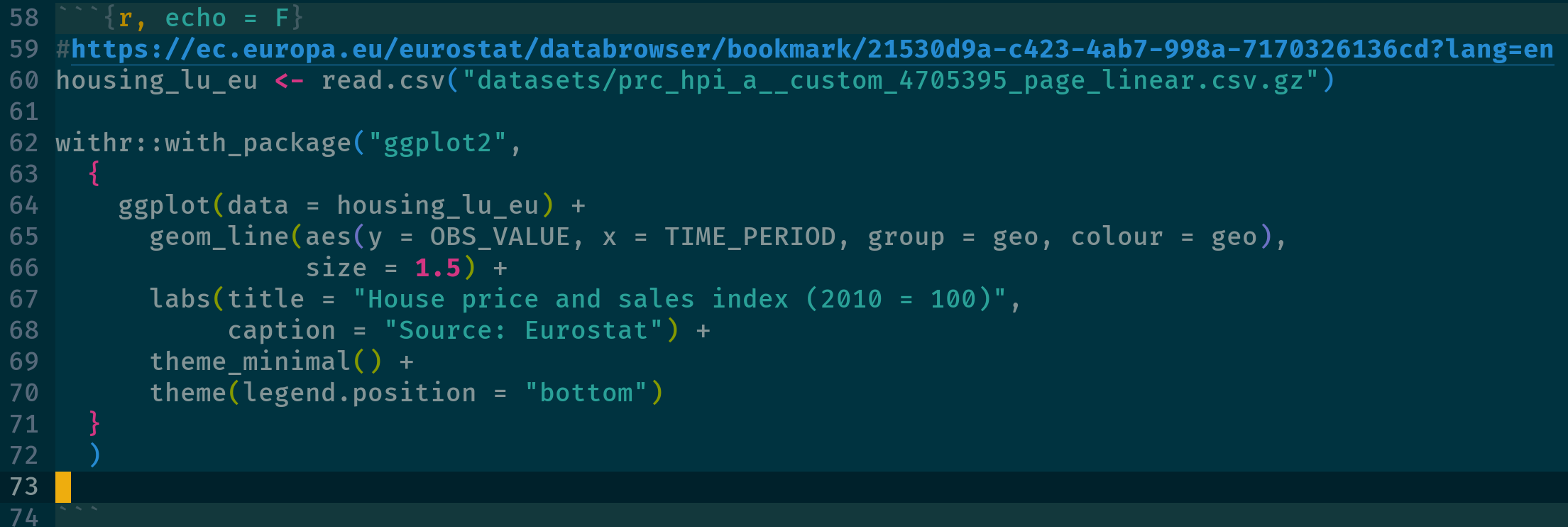
- Using library() will keep the package loaded during the whole session, with_package() just runs the code snippet with that package temporarily loaded. This can be useful to avoid namespace collisions for example
Read .csv from a zipped file
# long way
tmpf <- tempfile()
tmpd <- tempfile()
download.file('https://website.org/path/to/file.zip', tmpf)
unzip(tmpf, exdir = tmpd)
y <- data.table::fread(file.path(tmpd,
                       grep('csv$',
                            unzip(tmpf, list = TRUE)$Name,
                            value = TRUE)))
unlink(tmpf)
unlink(tmpd)

# quick way
y <- data.table::fread('curl https://website.org/path/to/file.zip | funzip')
Sometimes
curlwill fail with this error. To bypass the SSL issue, usecurl -k <url>curl: (60) SSL certificate problem: unable to get local issuer certificate More details here: https://curl.se/docs/sslcerts.html curl failed to verify the legitimacy of the server and therefore could not establish a secure connection to it.
Load all R scripts from a directory:
for (file in list.files("R", full.names = TRUE)) source(file)View dataframe in View as html table using {kableExtra}
df_html <- kableExtra::kbl(rbind(head(df, 5), tail(df, 5)), format = "html")
print(df_html)
Annotate interactively (source)
df <- data.frame( web = c("https://example.com/", "https://example.com/"), value = c(NA, NA) ) for (i in 1:nrow(df)) { if (is.na(df$value[i])) { browseURL(df$web[i]) df$value[i] <- menu(c("option A", "option B", "option C")) } }- Iterates through the df, opens the external link, and lets you add a value to a column in that row
Options
{readr}
options(readr.show_col_types = FALSE)
Cleaning
Misc
- Dates should follow YYYY-MM-DD format (ISO 8601 standard)
Remove all objects except:
rm(list=setdiff(ls(), c("train", "validate", "test")))Check if any column has above a certain percentage of NAs
Names of Columns
# matrix
na_cols <- colnames(mat)[colMeans(is.na(mat)) > 0.20]

# df
names(df)[colMeans(is.na(df)) > 0.20]
Matrices: All columns must be the same type (numeric, character, etc.)
Dataframes: Columns can be different types
Removal of Columns
# matrix
mat_clean <- mat[, !colnames(mat) %in% na_cols]
mat_clean <- mat[, colMeans(is.na(mat)) <= 0.20]

# df
df_clean <- df[, !names(df) %in% na_cols]
df_clean <- df[, colMeans(is.na(df)) <= 0.20]

df_clean <- df %>%
  janitor::remove_empty(which = "cols", prop = 0.20)

library(dplyr)
df_clean <- df %>%
  select(where(~ mean(is.na(.)) <= 0.20))
Remove/Replace NAs
See Lewis’s Recode NA tutorial for other options
Remove rows with any NAs
Dataframes
df %>% na.omit
df %>% filter(complete.cases(.))
df %>% tidyr::drop_na()
Variables
df %>% filter(!is.na(x1))
df %>% tidyr::drop_na(x1)
Remove rows will all NAs
df |> filter(!if_all(everything(), is.na))
df |> filter_out(if_all(everything(), is.na))
Replace NAs with 0 for certain columns (or the entire tibble w/
everything())d18 %>% dplyr::mutate(dplyr::across(Var1:Var2, ~ tidyr::replace_na(., 0)))- tidyselect functions are used to select particular sets of variables
Using
dplyr::replace_values(source)state <- c("NC", "NY", "CA", NA, "NY", "Unknown", NA) # Replace missing values with a constant replace_values(state, NA ~ "Unknown") #> [1] "NC" "NY" "CA" "Unknown" "NY" "Unknown" "Unknown" # Replace missing values with the corresponding value from another column region <- c("South", "North", "West", "East", "North", "Unknown", "West") replace_values(state, NA ~ region) #> [1] "NC" "NY" "CA" "East" "NY" "Unknown" "West" # Replace problematic values with a missing value replace_values(state, "Unknown" ~ NA) #> [1] "NC" "NY" "CA" NA "NY" NA NA # Standardize multiple issues at once replace_values(state, c(NA, "Unknown") ~ "<missing>") #> [1] "NC" "NY" "CA" "<missing>" "NY" "<missing>" #> [7] "<missing>"
Find duplicate rows
-
mtcars |> get_dupes(-c(wt, qsec)) #> mpg cyl disp hp drat vs am gear carb dupe_count wt qsec #> 1 21 6 160 110 3.9 0 1 4 4 2 2.620 16.46 #> 2 21 6 160 110 3.9 0 1 4 4 2 2.875 17.02 {datawizard} - Extract all duplicates, for visual inspection. Note that it also contains the first occurrence of future duplicates, unlike
duplicatedordplyr::distinct. Also contains an additional column reporting the number of missing values for that row, to help in the decision-making when selecting which duplicates to keep.df1 <- data.frame( id = c(1, 2, 3, 1, 3), year = c(2022, 2022, 2022, 2022, 2000), item1 = c(NA, 1, 1, 2, 3), item2 = c(NA, 1, 1, 2, 3), item3 = c(NA, 1, 1, 2, 3) ) data_duplicated(df1, select = "id") #> Row id year item1 item2 item3 count_na #> 1 1 1 2022 NA NA NA 3 #> 4 4 1 2022 2 2 2 0 #> 3 3 3 2022 1 1 1 0 #> 5 5 3 2000 3 3 3 0 data_duplicated(df1, select = c("id", "year")) #> 1 1 1 2022 NA NA NA 3 #> 4 4 1 2022 2 2 2 0{dplyr}
dups <- dat %>%
  group_by(BookingNumber, BookingDate, Charge) %>%
  filter(n() > 1)
base r
df[duplicated(df["ID"], fromLast = F) | duplicated(df["ID"], fromLast = T), ]

##        ID value_1 value_2 value_1_2
## 2  ID-003      6      5      6 5
## 3  ID-006      1      3      1 3
## 4  ID-003      1      4      1 4
## 5  ID-005      5      5      5 5
## 6  ID-003      2      3      2 3
## 7  ID-005      2      2      2 2
## 9  ID-006      7      2      7 2
## 10 ID-006      2      3      2 3
df[duplicated(df["ID"], fromLast = F)doesn’t include the first occurence, so also counting from the opposite direction will include all occurences of the duplicated rows
{tidydensity}
data <- data.frame(
  x = c(1, 2, 3, 1),
  y = c(2, 3, 4, 2),
  z = c(3, 2, 5, 3)
)

check_duplicate_rows(data)
#> [1] FALSE  TRUE FALSE FALSE
-
Remove duplicated rows
{datawizard} - From all rows with at least one duplicated ID, keep only one. Methods for selecting the duplicated row are either the first duplicate, the last duplicate, or the “best” duplicate (default), based on the duplicate with the smallest number of NA. In case of ties, it picks the first duplicate, as it is the one most likely to be valid and authentic, given practice effects.
df1 <- data.frame(
  id = c(1, 2, 3, 1, 3),
  item1 = c(NA, 1, 1, 2, 3),
  item2 = c(NA, 1, 1, 2, 3),
  item3 = c(NA, 1, 1, 2, 3)
)

data_unique(df1, select = "id")
#> (2 duplicates removed, with method 'best')
#>   id item1 item2 item3
#> 1  1     2     2     2
#> 2  2     1     1     1
#> 3  3     1     1     1
base R
df[!duplicated(df[c("col1")]), ]dplyr
distinct(df, col1, .keep_all = TRUE)
Replace Values
Also see R >> Base R >> Subsetting >> Value Replacement
{dplyr} (source)
df <-
  df |>
  mutate(across(where(is.numeric) & starts_with("CHI"),
                ~ case_when(
                  ID == 255 ~ NA,
                  .default = .)))
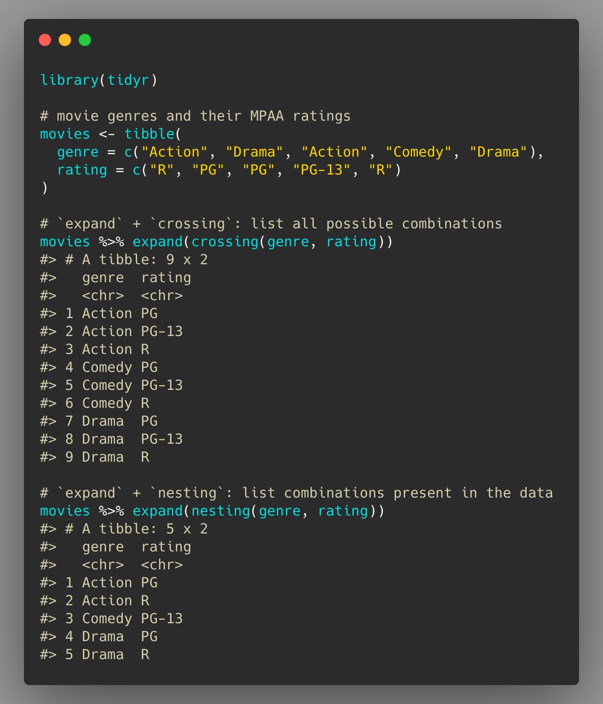
Showing all combinations present in the data and creating all possible combinations
Fuzzy Join
Packages
- {fozziejoin} - A modern, performance-oriented (Rust-based) alternative to {fuzzyjoin} (NOT a drop-in replacement but should have the same functionality)
- {fuzzyjoin} - Join tables together based not on whether columns match exactly, but whether they are similar by some comparison. Implementations include string distance and regular expression matching
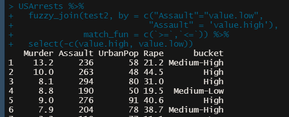
Example: {fuzzyjoin}
ref.df <- data.frame(
            bucket = c(“High”, “Medium-High”, “Medium-Low”, “Low”),
            value.high = c(max(USArrests$Assault), 249, 199, 149),
            value.low = c(250, 200, 150, min(USArrests$Assault)))

USArrests %>%
  fuzzy_join(ref.df,
             by = c("Assault"="value.low",
                    "Assault" = 'value.high'),
            match_fun = c(`>=`,`<=`)) %>%
  select(-c(value.high, value.low))
Also does partial matches
Remove NULL or empty elements from a list
ls_clean <-
      ls_dirty[!sapply(ls_dirty, \(x) is.null(x) || length(x) == 0)]

ls_clean <- Filter(Negate(is.null), ls_dirty)

ls_clean <- purrr::discard(x, ~ is.null(.x) || length(.x) == 0)
Remove elements of a list by name
purrr::discard_at(my_list, "a")
listr::list_remove
Filter row index before/after a condition
Example 1: Find flights that departed after an “AA” flight departed (article)
flights_df |>
  select(dep_time, flight, carrier) |>
  arrange(dep_time) |>
  slice(
    unique(sort(c(
      which(carrier == "AA"),
      which(carrier == "AA") + 1
    )))
  )
which(carrier == "AA")isn’t strictly necessary. It also includes AA flight that is proceded by the flight we’re looking for in case that’s something you also want to look at.- Without
sort, the output row order will have those strictly unnecessary AA flights first, then the flights we’re interested instead of them being in order of departure time.cwill contanenate the row indexes outputted by thewhichfunctions and sort will order them. This will result in the order being by departure time. - There’s a duplicate row, so
uniquegets rid of it.
Example 2: Get countries that are immediately before and after Germany in GDP for each year (article)
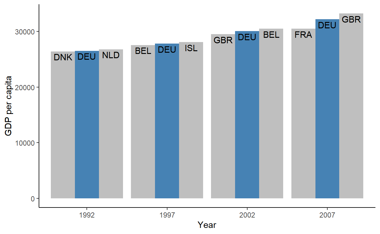
gdp_dat <- gapminder_df |>
  group_by(year) |>
  arrange(gdpPercap) |>
  slice(as.integer(outer(-1:1,
                         which(country == "Germany"),
                         `+` ))) |>
  # for ordering columns in plot
  mutate(grp = forcats::fct_inorder(c("lo", "is", "hi"))) |>
  # Ungroup and make ggplot
  ungroup()
* This assumes Germany will always have a country above and below it in GDP. See article for more robust code *
Instead using the syntax in the previous example where 1 is added to the index,
outeris used so that you don’t have to repeat a bunch ofwhichstatements.- -1:1 gets the rows before, after, and including the Germany row.
outerwith+stacks the vectors of indexes from each which statment on top of each other into a matrixas.integercoerces the matrix into a vector soslicecan filter the indexes.- See R, Base R >> Functions >> outer for a details on the
outerfunction
Chart code
Code
ggplot(gdp_dat,
       aes(as.factor(year),
           gdpPercap,
           group = grp)) +
  geom_col(aes(fill = grp == "is"), position = position_dodge()) +
  geom_text(
    aes(label = country_code),
    vjust = 1.3,
    position = position_dodge(width = .9)
  ) +
  scale_fill_manual(
    values = c("grey75", "steelblue"),
    guide = guide_none()
  ) +
  theme_classic() +
  labs(x = "Year", y = "GDP per capita")
Create labelled columns (source)
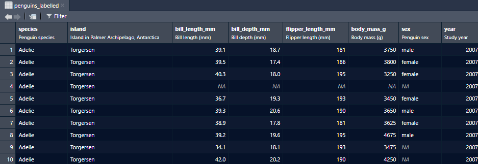
penguins_labelled <- penguins |>
  labelled::set_variable_labels(
    species           = "Penguin species",
    island            = "Island in Palmer Archipelago, Antarctica",
    bill_length_mm    = "Bill length (mm)",
    bill_depth_mm     = "Bill depth (mm)",
    flipper_length_mm = "Flipper length (mm)",
    body_mass_g       = "Body mass (g)",
    sex               = "Penguin sex",
    year              = "Study year"
  )
View(penguins_labelled)
Create a dictionary from the labelled df
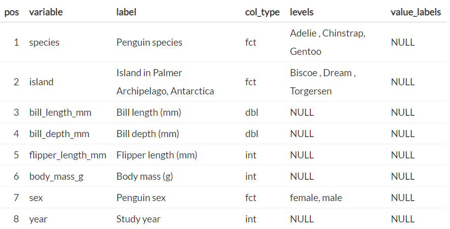
penguins_dictionary <- penguins_labelled |>
  labelled::generate_dictionary()
penguins_dictionary |>
  knitr::kable()
Transformations
- Dummy Encode (article)
Some modeling packages don’t accept factor variables and dummies must be explicitly provided.
dplyr
penguins_explicit <-
  reduce(
    levels(penguins$species)[-1],
    ~ mutate(.x, !!paste0("species", .y) := as.integer(species == .y)),
    .init = penguins
  )
.x provides the .init tibble and the successively recursed tibbles
To get a feel for what’s happening, here’s a simple illustration of the tidyevall bang-bang syntax plus walrus operator
new_cols <- c("a", "b", "c")
# add 3 cols called a,b,c with NAs
mtcars %>%
  head() %>%
  select(mpg) %>%
  mutate(!!new_cols[1] := NA) %>%
  mutate(!!new_cols[2] := NA) %>%
  mutate(!!new_cols[3] := NA)
data.table
penguins_dt <- as.data.table(penguins)

treatment_lvls <- levels(penguins_dt$species)[-1]
treatment_cols <- paste0("species", treatment_lvls)

penguins_dt[, (treatment_cols) := lapply(treatment_lvls, function(x){as.integer(species == x)})][]
Functions
Base-R unnest (source)
# nest all columns other than cyl and am into 'value'
x <- tidyr::nest(mtcars, value = -c(cyl, am))

#' tidyr-free unnest
#'
#' @param data nested tibble
#' @param cols string (max 1) identifying the nested column to be unnested
#'
#' @return unnested tibble, equivalant to tidyr::unnest(d, col)
unnest <- function(data, cols) {
  not_nested <- data[!names(data) == cols]
  nested <- data[cols]
  not_nested_expand <- not_nested[rep(seq_len(nrow(data)), sapply(nested[[cols]], nrow)), ]
  nested_expand <- do.call(rbind, nested[[cols]])
  res <- cbind(not_nested_expand, nested_expand)
  class(res) <- class(data)
  res
}

identical(tidyr::unnest(x, value), unnest(x, "value"))
#> [1] TRUE
Chunk a dataframe into equal portions
chunk_dat <- function(dat, n) { rows_per <- nrow(tib_comp) %/% (n-1) ls_split_dat <- split(dat, (seq(nrow(dat))-1) %/% rows_per) } my_tib_split <- chunk_dat(my_tib, 4)- Creates a list of 4 tibbles, each with similar (or same) number of rows
Create formula from string
analysis_formula <- 'Days_Attended ~ W + School'
estimator_func <- function(data) lm(as.formula(analysis_formula), data = data)
Recursive Function
Example
# Replace pkg text with html replace_txt <- function(dat, patterns) { if (length(patterns) == 0) { return(dat) } pattern_str <- patterns[[1]]$pattern_str repl_str <- patterns[[1]]$repl_str replaced_txt <- dat |> str_replace_all(pattern = pattern_str, repl_str) new_patterns <- patterns[-1] replace_txt(replaced_txt, new_patterns) }- Arguments include the dataset and the iterable
- Tests whether function has iterated through pattern list
- Removes 1st element of the list
replace_textcalls itself within the function with the new list and new dataset
Example: Using
RecallandtryCatchload_page_completely <- function(rd) { # load more content even if it throws an error tryCatch({ # call load_more() load_more(rd) # if no error is thrown, call the load_page_completely() function again Recall(rd) }, error = function(e) { # if an error is thrown return nothing / NULL }) }load_moreis a user defined functionRecallis a base R function that calls the same function it’s in.
Error Handling for Internal Functions (source)
library(cli) library(rlang) assert3 <- function(x, y, 1 arg = caller_arg(x), 2 call_expr = caller_call()) { 3 if (!inherits(x, y)) { 4 abort(format_error("{.strong {arg}} must be of class {y}"), 5 call = call_expr) } } some_fun3 <- function(x, class) { assert3(x, class) } some_fun3(5, "character") #> Error in `some_fun3()`: #> ! x must be of class character #> Run `rlang::last_trace()` to see where the error occurred. last_trace() #> <error/rlang_error> #> Error in `some_fun3()`: #> ! x must be of class character #> --- #> Backtrace: #> ▆ #> 1. └─global some_fun3(5, "character") #> 2. └─global assert3(x, class) #> Run rlang::last_trace(drop = FALSE) to see 1 hidden frame.- 1
-
rlang::caller_argformats the value of an argument (e.g. x) into a string so that can be used in error messages - 2
-
rlang::caller_call(with default being n = 1) goes 1 level up to get the function that called this function. - 3
-
inheritis a logical that tests whether x has the class indicated by y. Similar to anis.*function. - 4
-
cli::.strongadds bold text styling to the value - 5
-
call in
rlang::abortspecifies the environment to mention in the error message.
- By using
rlang::caller_callin the error function, the user will know which function in their script failed which is 1 level up from the assert (internal function). - Then
rlang::last_traceis used to drill down and discover that error was triggered in the internal function (e.g.assert3)
Calculations
Compute the running maximum per group
df <- structure(list(
  var = c(5L, 2L, 3L, 4L, 0L, 3L, 6L, 4L, 8L, 4L),
  group = structure(c(1L, 1L, 1L, 1L, 1L, 2L, 2L, 2L, 2L, 2L),
                    .Label = c("a", "b"),
                    class = "factor"),
  time = c(1L, 2L, 3L, 4L, 5L, 1L, 2L, 3L, 4L, 5L)),
  .Names = c("var", "group","time"),
  class = "data.frame",
  row.names = c(NA, -10L))

df[order(df$group, df$time),]
#    var group time
# 1    5    a    1
# 2    2    a    2
# 3    3    a    3
# 4    4    a    4
# 5    0    a    5
# 6    3    b    1
# 7    6    b    2
# 8    4    b    3
# 9    8    b    4
# 10  4    b    5

(df$curMax <-
  ave(df$var,
      df$group,
      FUN=cummax))

var  |  group  |  time  |  curMax
5      a        1        5
2      a        2        5
3      a        3        5
4      a        4        5
0      a        5        5
3      b        1        3
6      b        2        6
4      b        3        6
8      b        4        8
4      b        5        8
Time Series
Misc
- Resources
- Base R date-time manipulation with POSIXlt (hrbrmstr)
- Arithmetic, clamping, IANA zones, flexible handling of dates/time stamps
- Base R date-time manipulation with POSIXlt (hrbrmstr)
- R stores Date objects as the number of days since January 1, 1970 (Unix Epoch)
- Positive numbers: Represent dates after Jan 1, 1970.
- Negative numbers: Represent dates before Jan 1, 1970.
- Zero: Represents Jan 1, 1970, exactly
- Date origins used by other software
- R / Unix / Python - “1970-01-01”
- SAS / STATA - “1960-01-01”
- Excel (Windows, Modern Macs) - “1899-12-30”
- Excel (Older Macs) - “1904-01-01”
- MATLAB - “0000-01-01”
- Datetimes
- R uses 1970-01-01 00:00:00 UTC as it’s origin
- Similarly for other software origins except STATA which uses milliseconds
- Converting to a numeric vector is seconds since the origin (1 day = 86,400 secs)
- R uses 1970-01-01 00:00:00 UTC as it’s origin
Operations
Create a sequence of dates
Base
# Basic monthly sequence
dates <- seq.Date(
  as.Date("2023-01-01"),
  as.Date("2023-12-01"),
  by = "month"
)
# or equivalently
dates <- seq(
  as.Date("2023-01-01"),
  as.Date("2023-12-01"),
  by = "month"
)

# Create 12 monthly dates starting from Jan 2023
dates <- seq.Date(
  as.Date("2023-01-01"),
  by = "month",
  length.out = 12
)

# Last day of each month
dates_last <- seq.Date(
  as.Date("2023-01-31"),
  as.Date("2023-12-31"),
  by = "month"
)

# specific days
start_date <- as.Date("2023-01-01")
days_of_month <- c(15, 20, 10, 25, 5)

dates <- as.Date(paste0(
  format(start_date + months(0:4), "%Y-%m"),
  "-",
  days_of_month
))
Lubridate
dates <- seq(
  ymd("2023-01-01"),
  ymd("2023-12-01"),
  by = "month"
)

# Or with months() function
dates <- ymd("2023-01-01") %m+% months(0:11)

dates_last <- ceiling_date(
  seq(ymd("2023-01-01"),
      ymd("2023-12-01"),
      by = "month"),
  "month") - days(1)
Create a sequence of datetimes
Base
# Five hourly datetimes
seq(
  as.POSIXct("2023-01-15 09:30:00"),
  by = "hour",
  length.out = 5
)
#> [1] "2023-01-15 09:30:00 EST" "2023-01-15 10:30:00 EST" "2023-01-15 11:30:00 EST" "2023-01-15 12:30:00 EST"
#> [5] "2023-01-15 13:30:00 EST"

# specified intervals
seq(
  as.POSIXct("2023-01-15 12:00:00"),
  by = "30 min",  # or "7 days", "2 weeks", etc.
  length.out = 5
)
#> [1] "2023-01-15 12:00:00 EST" "2023-01-15 12:30:00 EST" "2023-01-15 13:00:00 EST" "2023-01-15 13:30:00 EST"
#. [5] "2023-01-15 14:00:00 EST"

# time zones
datetimes <- as.POSIXct(c(
  "2023-01-15 09:30:00",
  "2023-02-20 14:15:00",
  "2023-03-10 18:45:00",
  "2023-04-25 08:00:00",
  "2023-05-05 22:30:00"
), tz = "America/New_York")
Lubridate
# components
ymd_hms("2023-01-15 09:30:00") + minutes(0:4)
#> [1] "2023-01-15 09:30:00 UTC" "2023-01-15 09:31:00 UTC" "2023-01-15 09:32:00 UTC" "2023-01-15 09:33:00 UTC"
#> [5] "2023-01-15 09:34:00 UTC"

ymd_hms("2023-01-15 09:30:00") + hours(0:4) + minutes(0:4)
#> [1] "2023-01-15 09:30:00 UTC" "2023-01-15 10:31:00 UTC" "2023-01-15 11:32:00 UTC" "2023-01-15 12:33:00 UTC"
#> [5] "2023-01-15 13:34:00 UTC"

# more components
dates <- ymd(c("2023-01-15", "2023-02-20", "2023-03-10", "2023-04-25", "2023-05-05"))
times <- c("09:30:00", "14:15:00", "18:45:00", "08:00:00", "22:30:00")
datetimes <- ymd_hms(paste(dates, times))

# time zones
datetimes <- ymd_hms(c(
  "2023-01-15 09:30:00",
  "2023-02-20 14:15:00",
  "2023-03-10 18:45:00",
  "2023-04-25 08:00:00",
  "2023-05-05 22:30:00"
), tz = "UTC")
Converting between Date format and Numeric format
dates <- as.Date(c("1970-01-01", "2024-01-01", "1969-12-31"))
dates
#> [1] "1970-01-01" "2024-01-01" "1969-12-31"

num_dates <- as.numeric(dates)
#> [1]     0 19723    -1

# Converting back to Date objects
as.Date(num_dates, origin = "1970-01-01")
#> [1] "1970-01-01" "2024-01-01" "1969-12-31"
Converting between Datetime format and Numeric format
datetime <- as.POSIXct("2026-02-19 10:35:00", tz = "UTC")

(num_datetime <- as.numeric(datetime))
#> [1] 1771497300

as.POSIXct(num_datetime, origin = "1970-01-01", tz = "UTC")
#> [1] "2026-02-19 10:35:00 UTC"

# lop off milliseconds when included (13 digits)
as.POSIXlt(as.numeric(
  # paste converts to string
  substr(paste(data$generation_time[1]),
         start = 1,
         stop = 10)),
  origin = "1970-01-01")
#> [1] "2011-10-14 11:14:46 CEST"
The previous month and its year (source)
library(lubridate)
prev_month <-
  add_with_rollback(today(), months(-1)) |>
  month(label = TRUE, abbr = FALSE)

prev_months_yr <-
  add_with_rollback(today(), months(-1)) |>
  year()

# base r
format(seq(Sys.Date(), length = 2, by = "-1 month")[2], "%B %Y")
Subsetting
Base
# rows
sub_data <-
  data[data$TIME >= as.POSIXct('2011-12-12 00:00 CET') &
         data$TIME <= as.POSIXct('2011-12-14 23:00 CET'), ]

# columns
# dates is a vector of dates in same order as the columns of air
keep_cols <- dates >= as.Date("2005-01-01") &
  dates <= as.Date("2010-12-31")

air_sub <- air[, keep_cols]
Intervals
Difference between dates
# Sample dates
start_date <- as.Date("2022-01-15")
end_date <- as.Date("2023-07-20")

# Calculate time difference in days
time_diff_days <- end_date - start_date

# Convert days to months
months_diff_base <- as.numeric(time_diff_days) / 30.44  # average days in a month

cat("Number of months using base R:", round(months_diff_base, 2), "\n")
#> Number of months using base R: 18.1
Moving Windows
- Example (article)
For each 3 day window:
- Find the minimum value
- Find the time of the minimum value
- Find the value of two other columns at that time of the minimum value
Code
(ts_df <- tibble( time = 1:6, val = sample(1:6 * 10), col1 = rnorm(6), col2 = rnorm(6) )) #> # A tibble: 6 × 4 #> time val col1 col2 #> <int> <dbl> <dbl> <dbl> #> 1 1 10 -0.529 0.928 #> 2 2 30 0.874 -0.967 #> 3 3 60 1.50 1.49 #> 4 4 40 -1.14 0.575 #> 5 5 20 0.114 0.307 #> 6 6 50 -0.712 -0.291 moving_mins <- ts_df |> slice( outer(-2:0, row_number(), "+")[,-(1:2)] |> apply(MARGIN = 2L, \(i) i[which.min(val[i])]) ) |> rename_with(~ paste0("min3val_", .x)) |> mutate(time = ts_df$time[-(1:2)]) left_join(ts_df, moving_mins, by = "time") #> time val col1 col2 min3val_time min3val_val min3val_col1 min3val_col2 #> <int> <dbl> <dbl> <dbl> <int> <dbl> <dbl> <dbl> #> 1 1 10 -0.529 0.928 NA NA NA NA #> 2 2 30 0.874 -0.967 NA NA NA NA #> 3 3 60 1.50 1.49 1 10 -0.529 0.928 #> 4 4 40 -1.14 0.575 2 30 0.874 -0.967 #> 5 5 20 0.114 0.307 5 20 0.114 0.307 #> 6 6 50 -0.712 -0.291 5 20 0.114 0.307- See article for in-depth breakdown of what the code is doing.
outercreates a column-wise lagged matrix- Also see Cleaning >> Filter row index before/after a condition >> Example 2 which gives more detail on what’s happening with
outer
- Also see Cleaning >> Filter row index before/after a condition >> Example 2 which gives more detail on what’s happening with
applyloops through each column and selects the index of the minimum valueslicefilters the dateset for those indexes- Everything else is just adding columns back from the original df
- Example (article)