General
Misc
- Packages
- {brulee} - {tidymodels} interface to {torch}
- Contains several basic modeling functions that use the torch package infrastructure, such as: neural networks, linear regression, logistic regression, and multinomial regression.
- {keras} - R interface to keras
- {kindling} (overview, bayesian) - A higher-level interface built on top of {torch}
- Multiple architectures available: feedforward networks (MLP/DNN/FFNN) and recurrent variants (RNN, LSTM, GRU)
- Native support for titanic ML frameworks (currently supports {tidymodels} (and {mlr3} soon) workflows and pipelines
- {luz} - A higher level API for {torch} providing abstractions to allow for much less verbose training loops
- {mlr3torch} - Deep Learning with {torch} and {mlr3}
- {torch} - R interface to Torch
- {brulee} - {tidymodels} interface to {torch}
- Resources
- Deep Learning and Scientific Computing with R torch
- Tensorflow for R
- Hands-On Machine Learning With R, Ch. 13 - Deep learning with {keras}
- Guide for suitable baseline models: link
- DL model cost calculator (github) (article)
- Use Adam and AdamW optimizers
- Always log the L1 norm of the gradient when using Adam! It’s far more informative than the L2 norm - it better indicates convergence issues, and it’s more stable. (link)
- Keras also provides out-of-the-box preprocessing layers. This way, when the model is saved, the preprocessing steps will automatically be part of the model.
- i.e. The same preprocessing steps applied in training are applied in production
- But preprocessing steps will be wastefully repeated on each iteration through the training dataset. The more expensive the computation, the more this adds up.
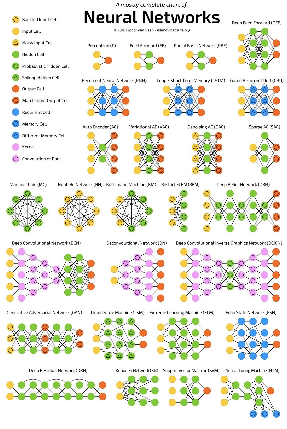
- DL architectures
Terms
- Activation Function: After the node calculates the weighted sum of the input, the activation function transforms the output which is fed to the next layer.
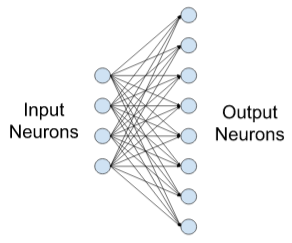
- Fully-Connected Layers (aka Linear Layers) - Connect every input neuron to every output neuron. Each neuron applies a linear transformation to the input vector through a weights matrix. As a result, all possible connections layer-to-layer are present, meaning every input of the input vector influences every output of the output vector. Three parameters define a fully-connected layer: batch size, number of inputs, and number of outputs. (see article)
- Modalities
- Unimodal Models: text-only, image-only, etc.
- Multimodal Models: text, image, continuous sensor data, etc.
- Mini-Batch Gradient Descent - The algorithm randomly selects a group of data points (batch) and uses it to update the parameter values, instead of using the entire dataset as in Gradient Descent or just one row of data as in Stochastic Gradient Descent.
- Stochastic Gradient Descent - The algorithm randomly selects a single row of data and uses it to update the parameter values, instead of using the entire dataset as in Gradient Descent. A much faster method that Gradient Descent.
Basic Feed Forward
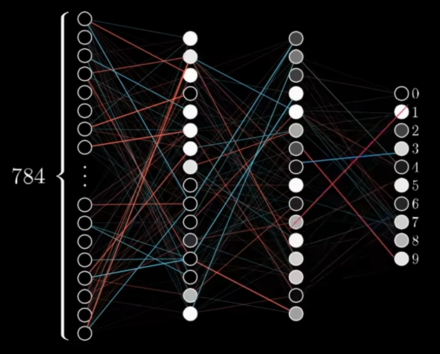
- Notes from 3Blue1Brown series which uses the MNIST dataset and a neural network with 2 hidden layers with sigmoid activation functions (transform values to be between 0 and 1) and softmax output layer (probabilites).
Structure
- An image is matrix where each cell has a brightness value
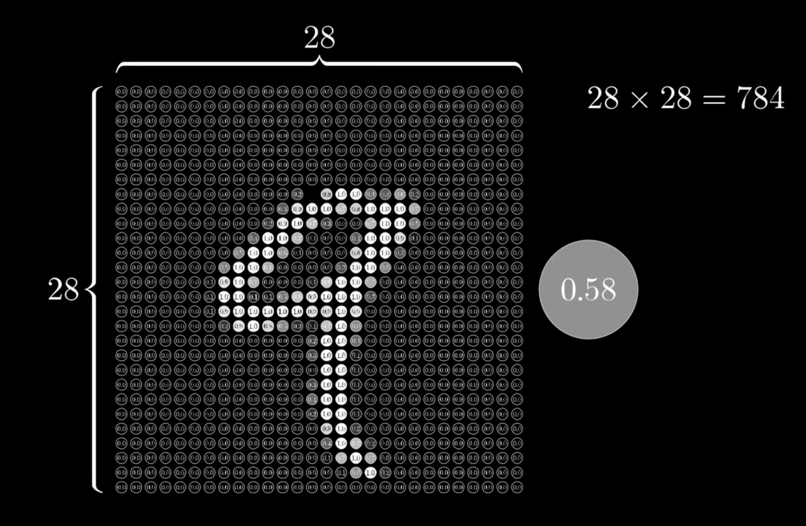
- There will be 784 input values for the first hidden layer.
- 0.58 is one of brightness values that was at the top of the “9”
- The activation equation for one neuron/node
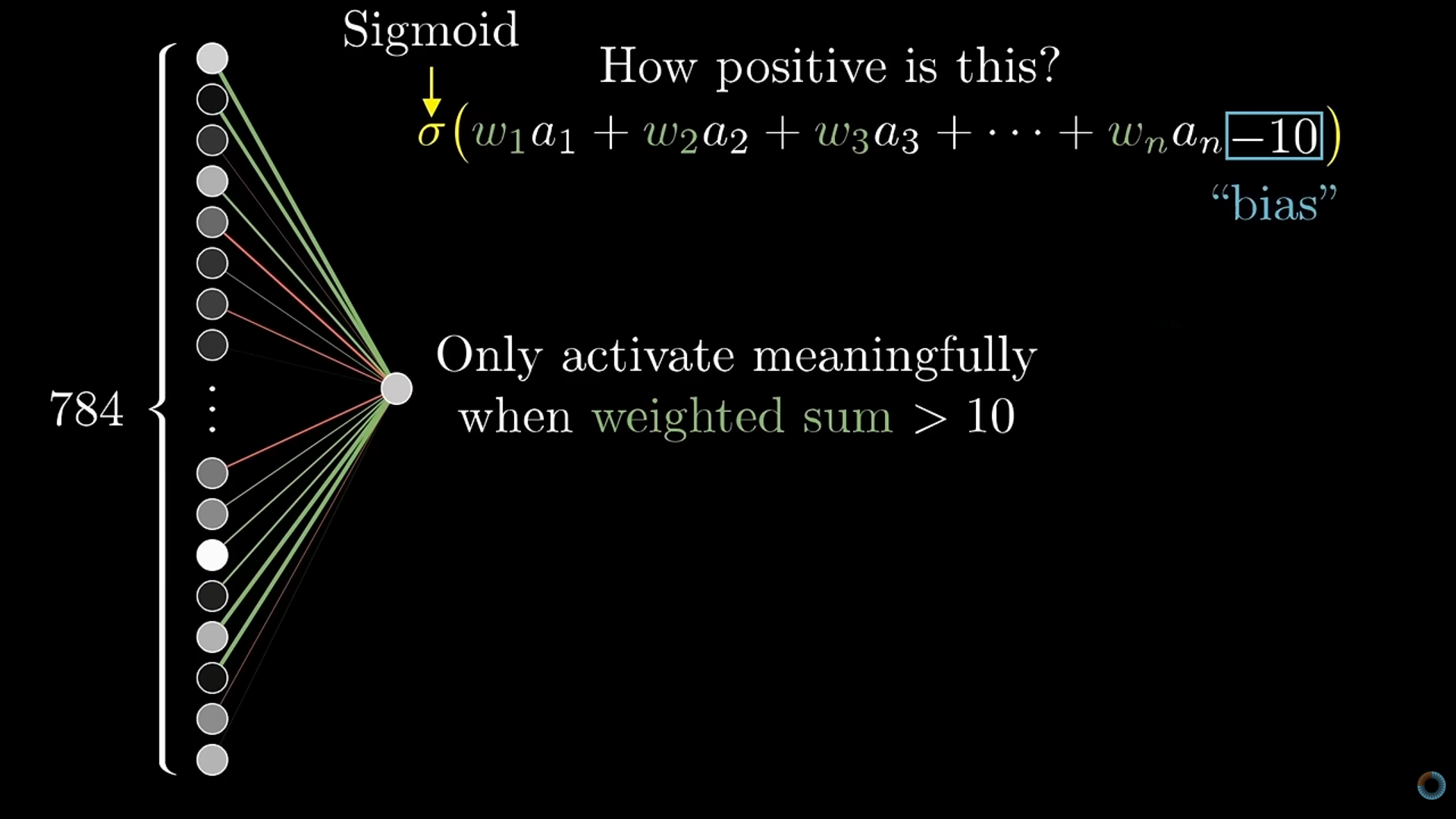
- This equation produces the activation value for one neuron
- \(w_i\) are the weights and -10 is the bias (\(b_i\)). These are parameters that get optimized in each layer
- The -10 bias value says the weighted sum needs to be greater than 10 for the neuron to be “activated.”
- The weighted sum plus bias is essentially just a regression equation which is fed into the sigmoid (activation function) which transforms it into a value between 0 and 1
- The activation equation for one layer
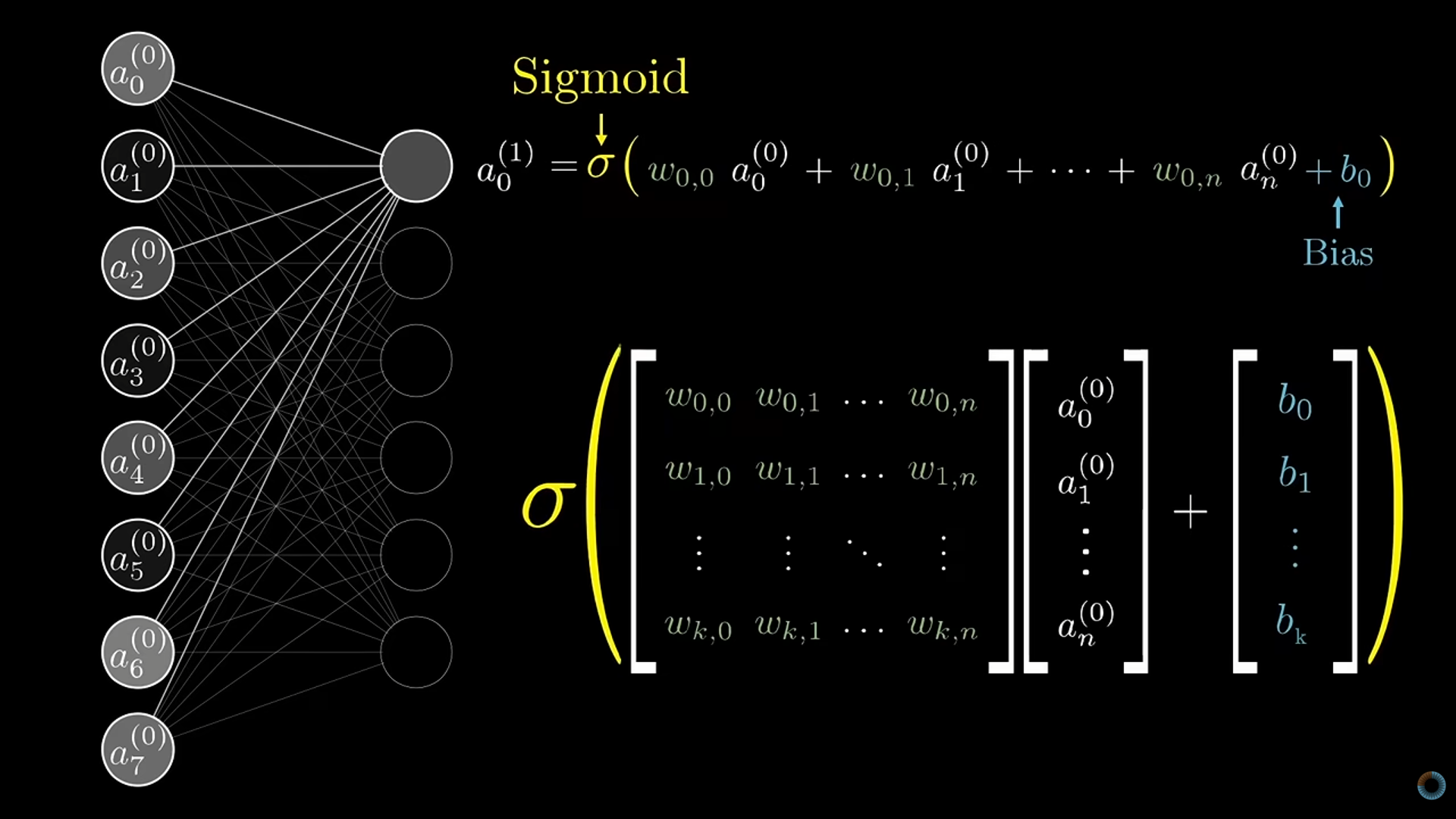
- Each row in the weights matrix is a neuron (e.g. 2nd row is the 2nd neuron)
- For the first fully connected hidden layer, there will be 784 weights and 1 bias value for each node. If there are 16 neurons in this hidden layer, then this layer has (784 x 16) + 16 = 12,560 parameters.
- Overall
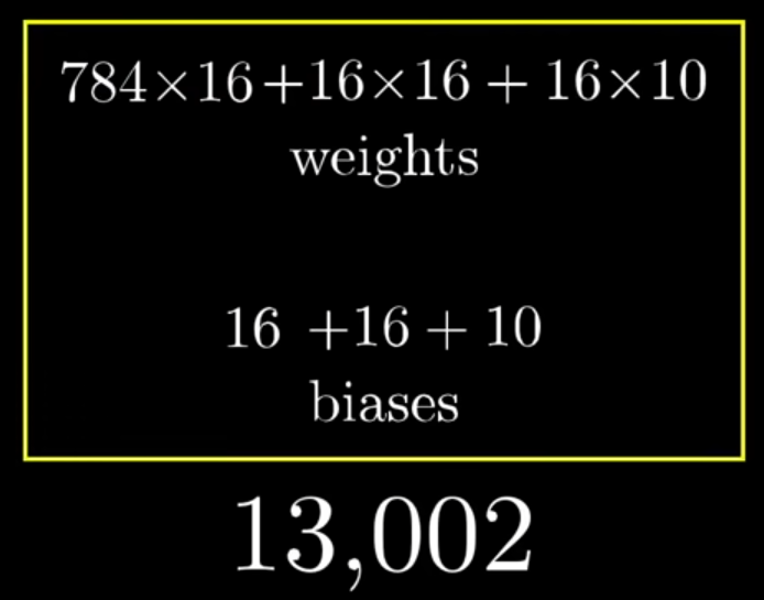
- Since it’s the second hidden layer, there’s only 16 inputs (activation values), so it’s 16 x 16 total weights. Then the last layer, which is a softmax, has the 10 possible numbers in MNIST. With the biases, this gives a grand total of 13,002 parameters that need to be estimated.
Gradient Descent
Method used to select weight and bias values that minimize a cost function
Cost Function
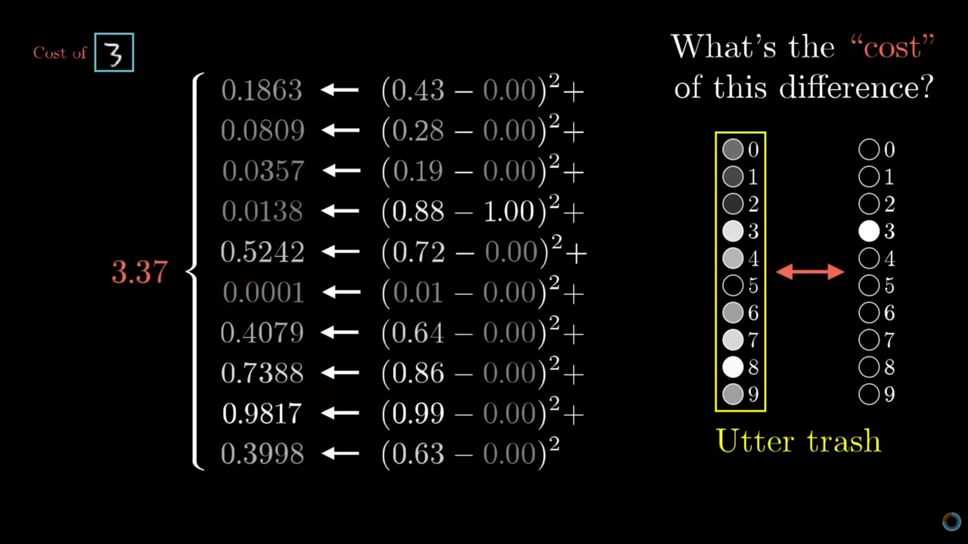
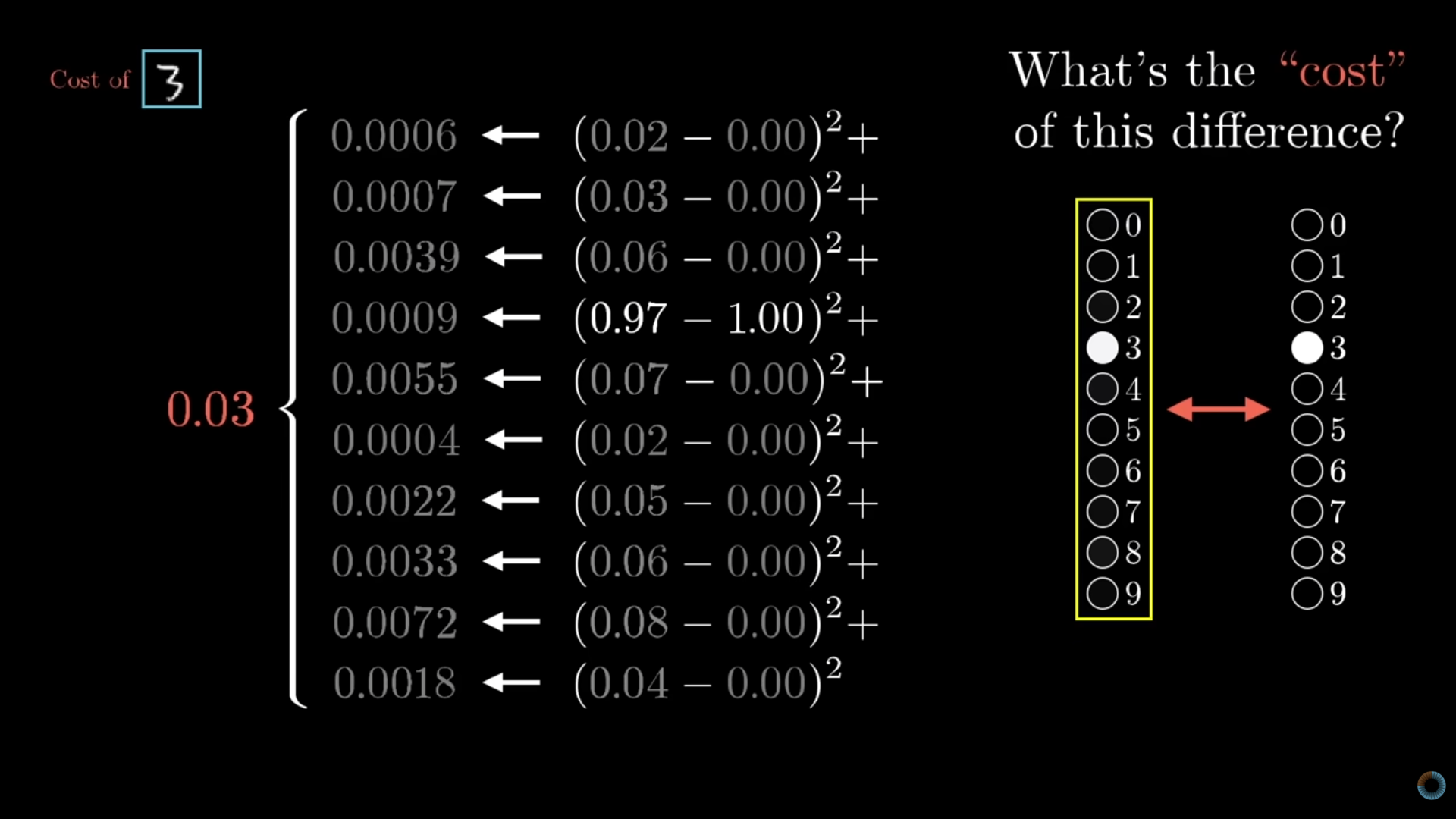
- Left: Shows a network after 1 epoch which has a brier score of 3.37. This is the average of the squared differences between the predicted probability and the truth.
- Right: Shows a trained network that has brier score of 0.03.
- The Brier Score is the cost function that we want to minimize
Simple 1-D Illustration
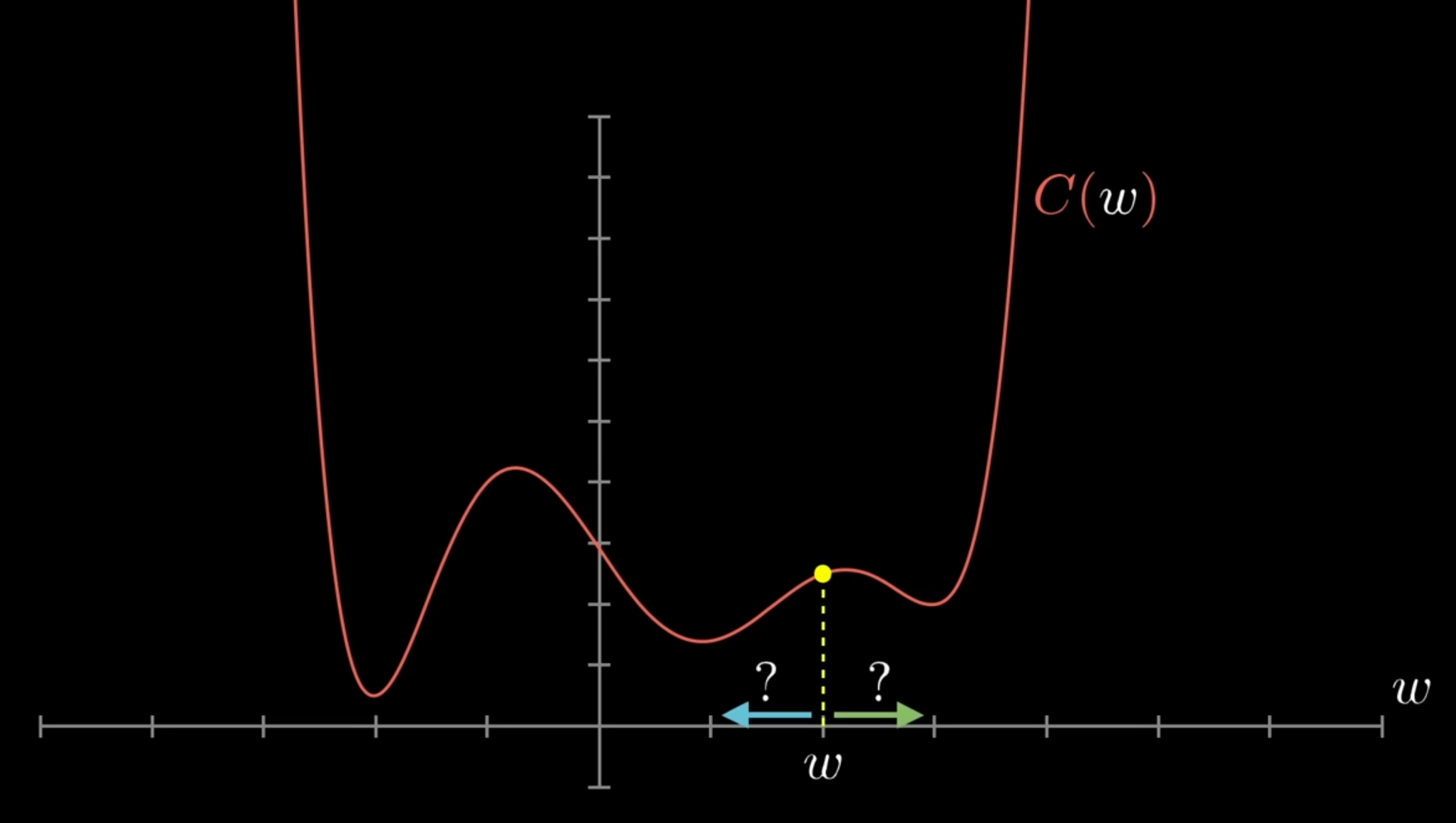
- The cost is the Y-axis and the weight value is the X-axis
- Left: If the cost is some value, how do we mathematically find out whether we should lessen the weight value or increase it?
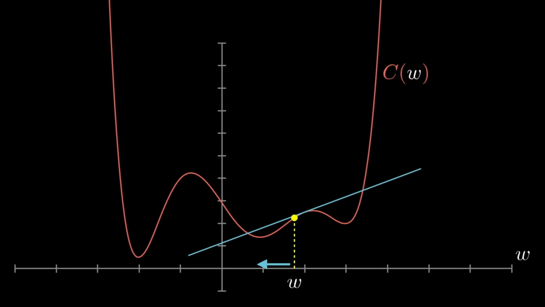
- Right: By taking the derivative of the Cost function with respect to \(w\) and plugging in \(w\), we get a positive value. This value is of course the slope of the tangent at that point.
- Since the slope is positive, we know to lessen the weight value in order to move towards a local minimum of the cost function
Simple 3-D Illustration
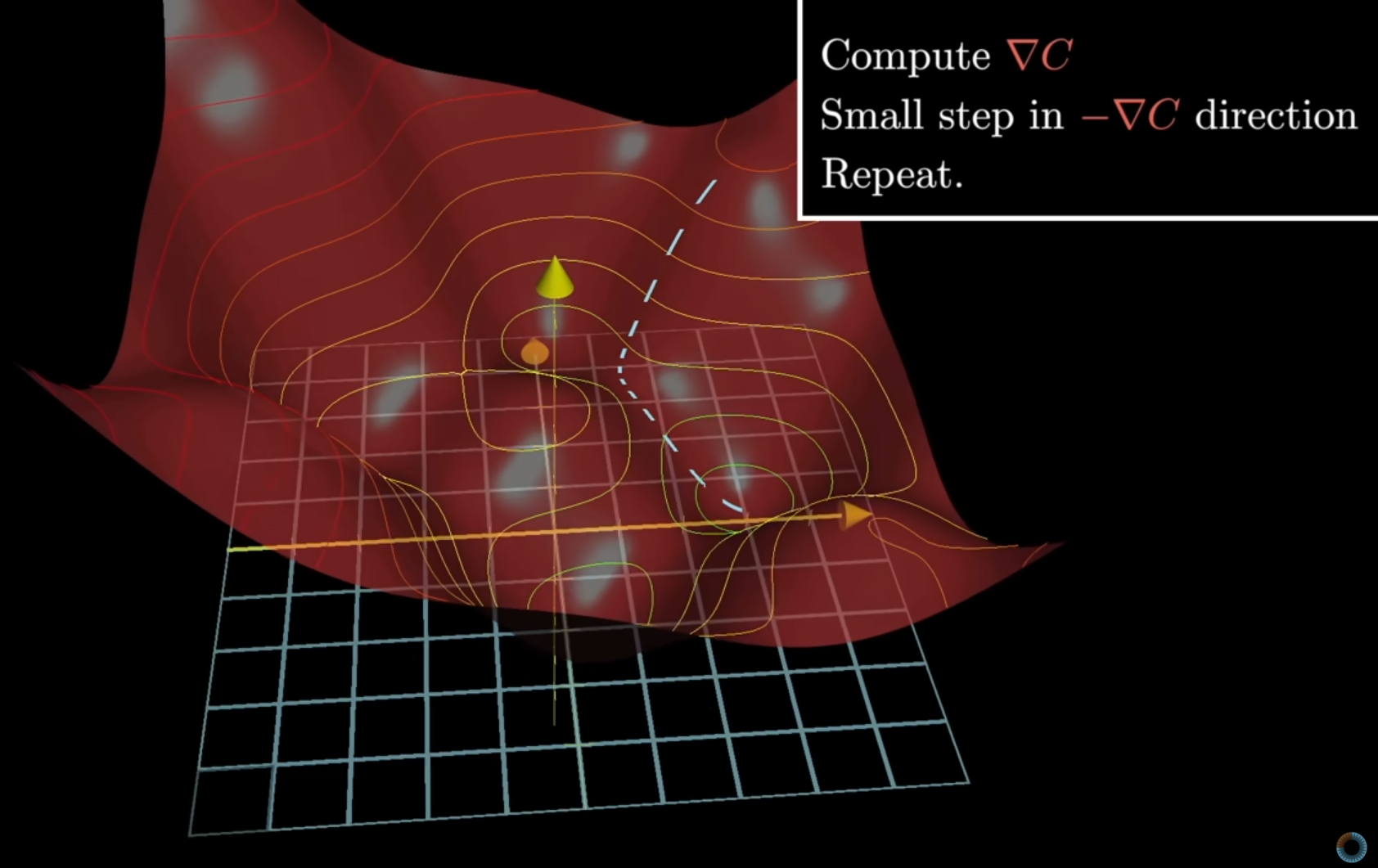
- This visualizes, in general, the process in which the gradient descent method takes steps (learning rate) towards a local minimum of the cost function (where \(\Delta C\) is the gradient)
The gradient the weights vector tells us how to adjust the weights.
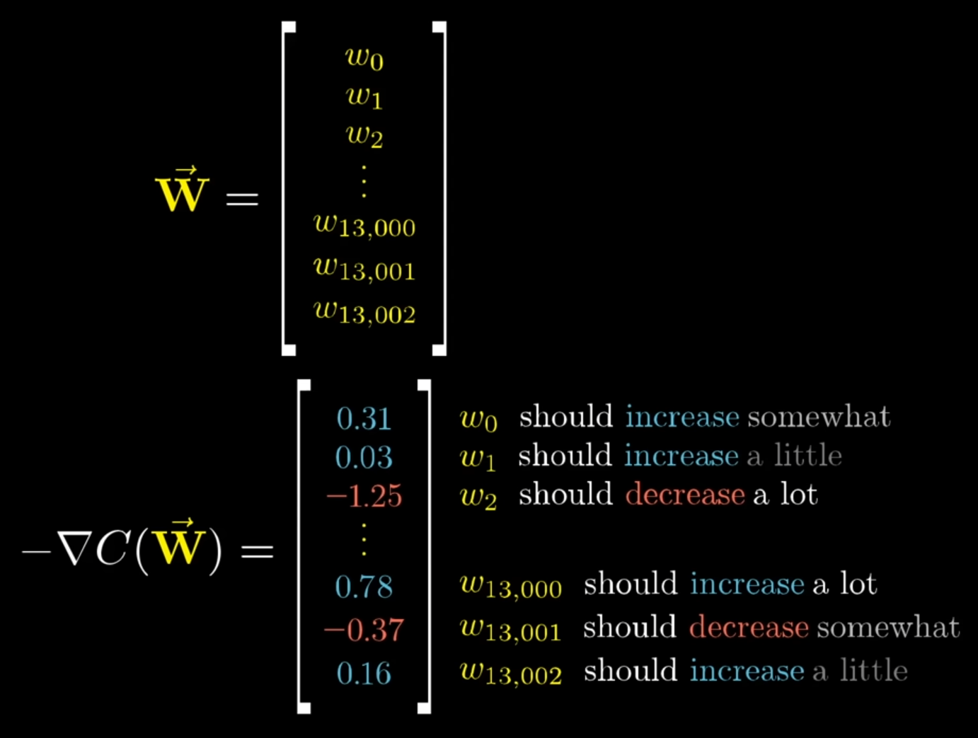
- The negative of the gradient is the value that should be added to weight.
- This is also used to adjust the bias value
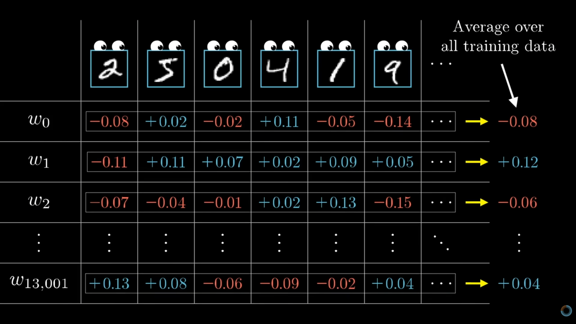
- The gradient values that get applied to the weights are actually averages of the gradients calculated across all images in the training data.
- A nudge to weight with a gradient of 3.20 has 32 times more influence on the cost than a weight with a gradient of 0.10.
- The negative of the gradient is the value that should be added to weight.
Backpropagation Math
AKA Backward Pass. The process by which all the weights and biases get adjusted using the gradients.
Overview
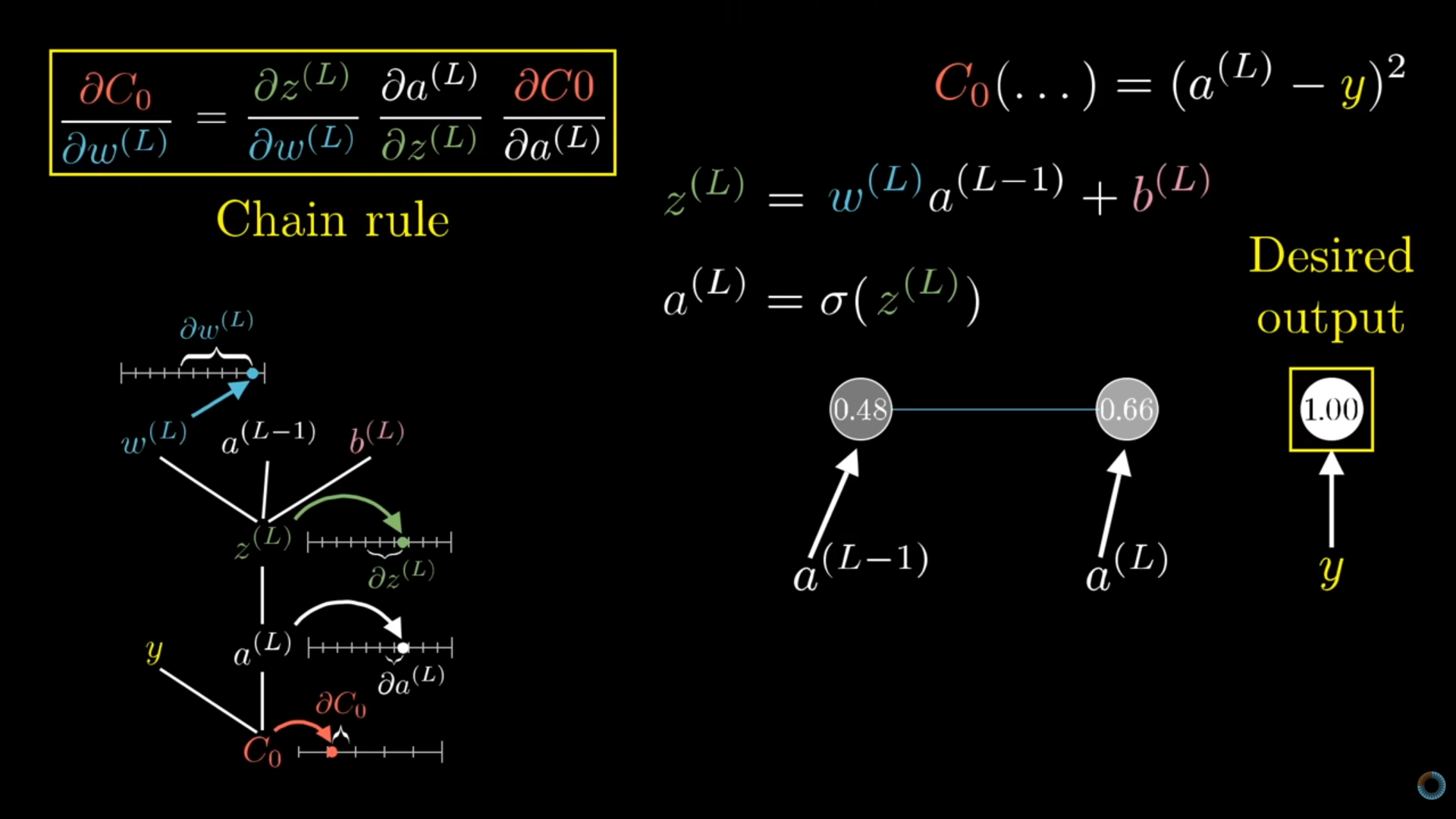
- Bottom Right: For simplicity, only one neuron’s/node’s activation value from the last hidden layer (\(a^{(L-1)}\)) and the output layer (\(a^{(L)}\)) are used
- Left Bottom: Shows the parameters (weights, bias, activation values) and the hierarchical nature (chain rule) of the gradient calculation.
- Ignore the little number lines. They were for animating how the change in one parameter affected others below it.
- Left Top: Shows the calculation of the weight gradient that gets used to calculate the final activation value before it gets fed into the softmax function
- Top Right: Shows the equations used in the derviative calculations — the cost function (\(C_0\)), the weighted sum (weights, biases) (\(z^{(L)}\)), and the full activation value equation (\(a^{(L)}\)) that includes the activation function (sigmoid in this case).
Calculate Derivatives
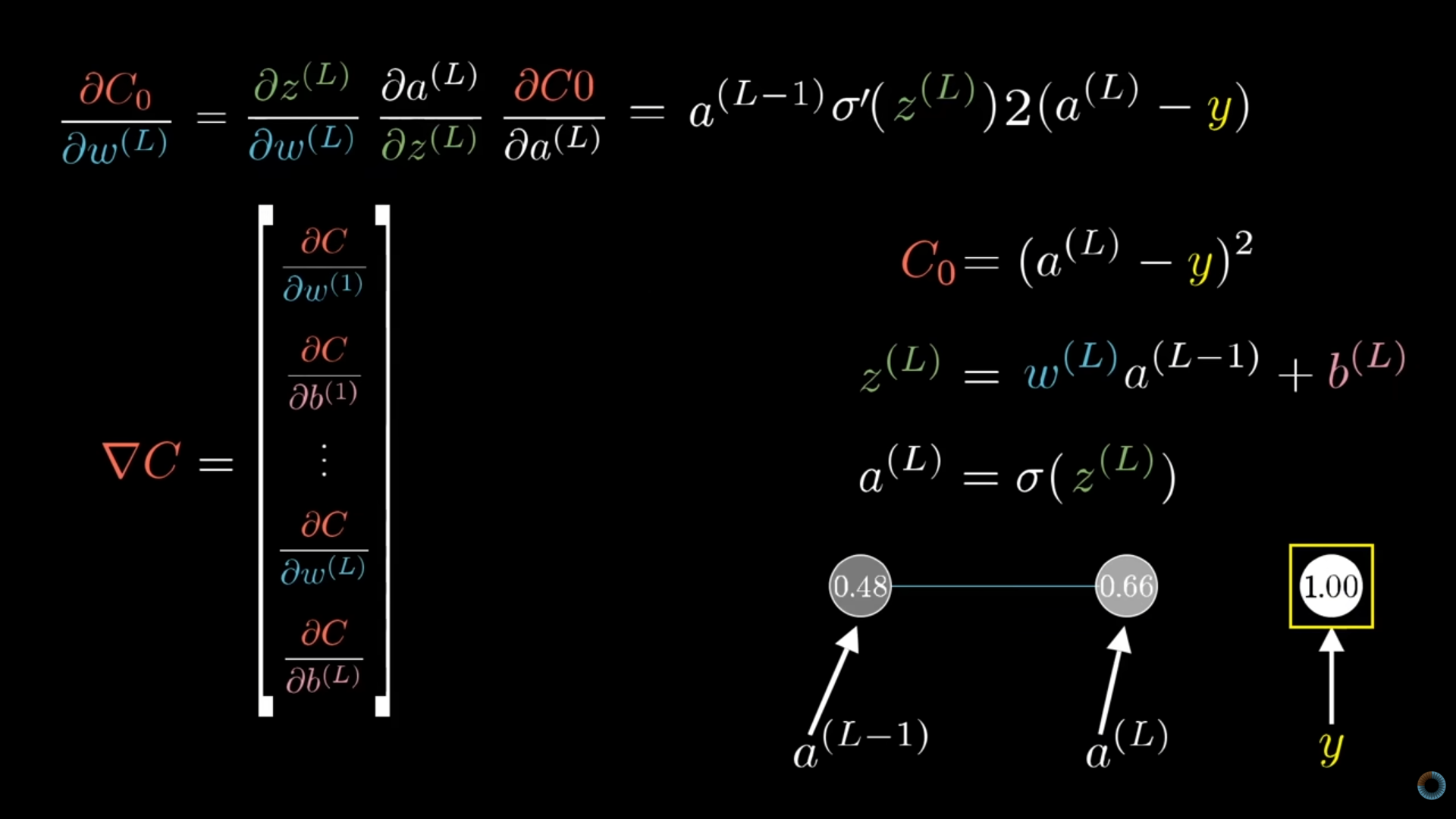
- Top: Shows the derivatives of the components for the gradient for the weights
- Bottom Left: Just shows the whole gradient vector that includes all the neurons/nodes and gradients for weights and biases
- The gradient for the bias is very similar. You just replace \(\frac{\partial z^{(L)}}{\partial w^{(L)}}\) with \(\frac{\partial z^{(L)}}{\partial b^{(L)}}\) in the chain rule equation. This results in a derivative equal to 1 instead of \(a^{(L-1)}\).
- Remember, that actually, the gradients in the gradient vector would be averages of gradients across all images (samples) in the training data.
Activation functions
- Misc
- The choice of activation function has a large impact on the capability and performance of the neural network, and
- Different activation functions may be used in different layers of the model.
- Commonly the same activation function is used for the hidden layers and a different one for the outer layer that makes the prediction (e.g. softmax)
- Most activation functions add non-linearity to the neural network
- Both the sigmoid and Tanh functions can make the model more susceptible to problems during training, via the so-called vanishing gradients problem.
- Architectures
- Hidden layers
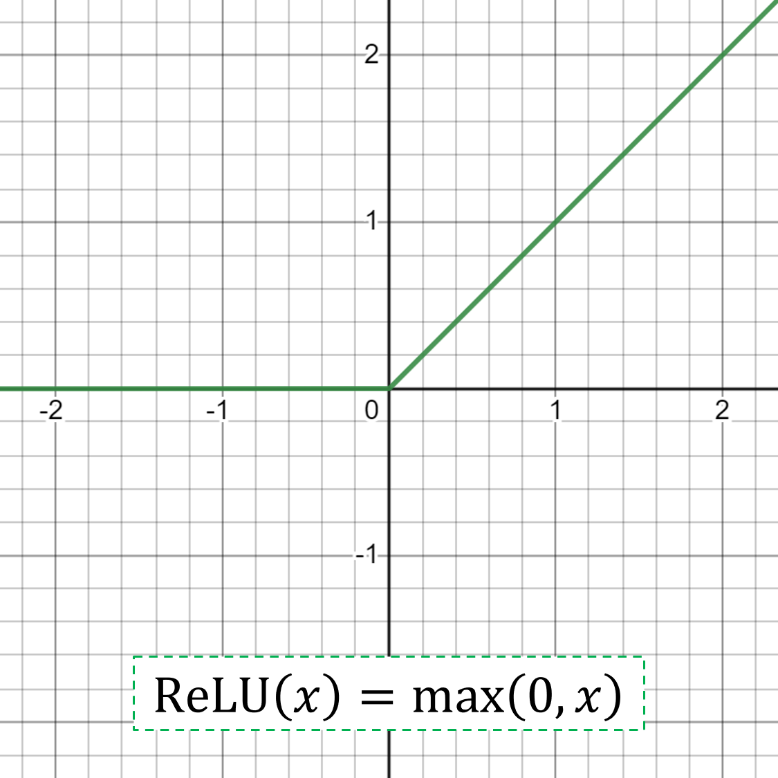
- Multilayer Perceptron (MLP): ReLU activation function.
- Convolutional Neural Network (CNN): ReLU activation function.
- Recurrent Neural Network (RNN): Tanh and/or Sigmoid activation function
- Outer layer
- Regression: One node, linear activation
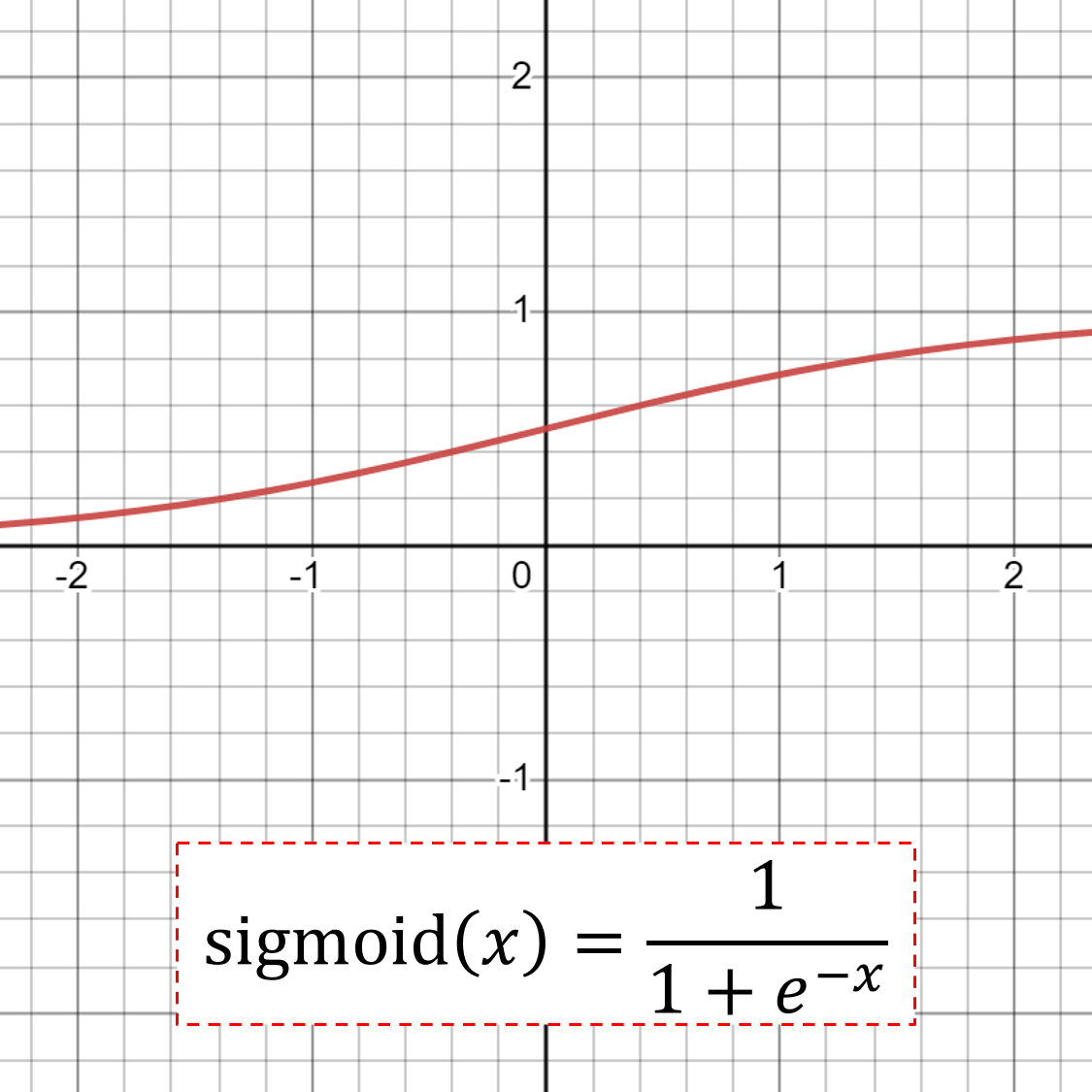
- Binary Classification: One node, sigmoid activation.
- Multiclass Classification: One node per class, softmax activation.
- Multilabel Classification: One node per class, sigmoid activation.
- Hidden layers
- Base Types
- ReLU: if the input value (x) is negative, then a value 0.0 is returned, otherwise, the value is returned
- Sigmoid: Logistic function; output is 0 to 1
- A perceptron is called the logistic regression model if the activation function is sigmoid.
- Good practice to use a “Xavier Normal” or “Xavier Uniform” weight initialization (aka Glorot initialization)) and scale input data to the range 0-1 (e.g. the range of the activation function) prior to training.
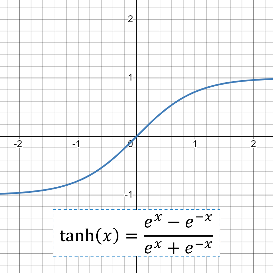
- tanh: takes any real value as input and outputs values in the range -1 to 1
- The larger the input (more positive), the closer the output value will be to 1.0, whereas the smaller the input (more negative), the closer the output will be to -1.0.
- Good practice to use a “Xavier Normal” or “Xavier Uniform” weight initialization (aka Glorot initialization) and scale input data to the range -1 to 1 (e.g. the range of the activation function) prior to training.
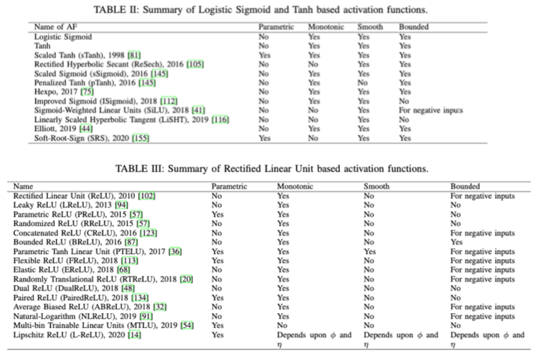
- Comprehensive Survey and Performance Analysis of Activation Functions in Deep Learning, paper
Regularization
- Misc
- Other methods
- Data Augmentation
- More data reduces variance
- Computer vision: Gain data by flipping, zooming, and translating the original images
- Digits Recognition: Gain data by mposing distortion on the images
- Early Stopping
- Stopping the training phase before a defined number of iterations
- For an overfitting model, if we plot the cost function on both the training set and the validation set as a function of the iterations.
- The training error always keeps decreasing but the validation error might start to increase after a certain number of iterations.
- When the validation error stops decreasing, that is exactly the time to stop the training process.
- By stopping the training process earlier, we force the model to be simpler, thus reducing overfitting.
- Data Augmentation
- Other methods
- L1 and L2 regularization
- Shrinks model weights
- Regularization process
- The weights of some hidden units become closer (or equal) to 0. As a consequence, their effect is weakened and the resulting network is simpler because it’s closer to a smaller network. As stated in the introduction, a simpler network is less prone to overfitting.
- For smaller weights, also the input z of the activation function of a hidden neuron becomes smaller. For values close to 0, many activation functions behave linearly.
- L2 regularization may not be necessary to achieve a highly accurate model when applying batch normalization or dropout but Guo et al. empirically demonstrated the model tends to be less calibrated without using L2 regularization. (source)
- L1
Cost Function, J
\[J(w^{[1]}, b^{[1]}, \ldots, w^{[L]}, b^{[L]}) = \frac{1}{m}\sum_{i=1}^m \mathcal{L}(\hat{y}^{(i)}, y^{(i)}) + \frac{\lambda}{2m} \sum_{l=1}^L \lVert w^{[l]} \rVert_1\]
- \(\mathcal{L}\): Loss Function
- \(m\): Number of Training Observations (aka Examples)
- \(w\) and \(b\): The weight and bias terms in the output of the node respectively
Regularization term
\[\frac{\lambda}{2m} \sum_{l=1}^L \lVert w^{[l]} \rVert_1\]
\(L\): The number of layers
\(\lambda\): Regularization Factor
\(w\): The norm of the weights
\[\lVert w^{[l]} \rVert_1 = \sum_i \sum_j |w_{i,j}^{[l]}|\]
- L2
Same as L1 except for the regularization term
Regularization term
\[\frac{\lambda}{2m} \sum_{l=1}^L \lVert w^{[l]} \rVert_2^2\]
\(w\): The norm of the weights
\[\lVert w^{[l]} \rVert_2^2 = \sum_i \sum_j (w_{i,j}^{[l]})^2\]
- Dropout
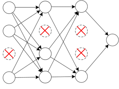
- Randomly remove some nodes in the network
- Performed separately for each training example.
- Therefore, each training example might be trained on a different network.
- Regularization Process
- Has the effect of temporarily transforming the network into a smaller one, and we know that smaller networks are less complex and less prone to overfitting.
- Because some of its inputs may be temporarily shut down due to dropout, the unit can’t always rely on them during the training phase. As a consequence, the hidden unit is encouraged to spread its weights across its inputs. Spreading the weights has the effect of decreasing the squared norm of the weight matrix, resulting in a sort of L2 regularization.
- Process
- Set a probability, p, for each node of the network.
- Typically, the keeping probability is set separately for each layer of the neural network
- For layers with a large weight matrix, a smaller keeping probability because, at each step, we want to conserve proportionally fewer weights with respect to smaller layers
- During the training phase, each node has a p probability to be turned off.
- Set a probability, p, for each node of the network.
- Randomly remove some nodes in the network
Ablation Testing
- Tests to evaluate how robust DL models are to different kinds of disruption.
- Misc
- Notes from Ablation Testing Neural Networks: The Compensatory Masquerade
- Similar to hyperparamter tuning with the goal of optimization except Ablation Testing is more about changing the architecture of the ANN (e.g. neurons, layers, etc), where as hyperparameter tuning refers to changing structural parameters of the model.
- Use Cases
- Identifying Critical Parts of a Neural Network
- Some parts of a neural network may do more important work than other parts of a neural network. In order to optimize the resource usage and the training time of the network, we can selectively ablate “weaker learners”
- Reducing Complexity of the Neural Network
- Sometimes neural networks can get quite large, especially in the case of Deep MLPs (multi layer perceptrons). This can make it difficult to map their behavior from input to output. By selectively shutting of parts of the network, we can potentially identify regions of excessive complexity and remove redundancy — simplifying our architecture.
- Fault Tolerance
- In a realtime system, parts of a system can fail. The same applies for parts of a neural network, and thus the systems that depend on their output. Ablation studies can determine if destroying certain parts of the neural network, will cause the predictive or generative power of the system to suffer.
- Identifying Critical Parts of a Neural Network
- Types
- Neuronal Ablation: Remove varying percentages of neurons from our neural network (i.e. dropout rate)
- Example:
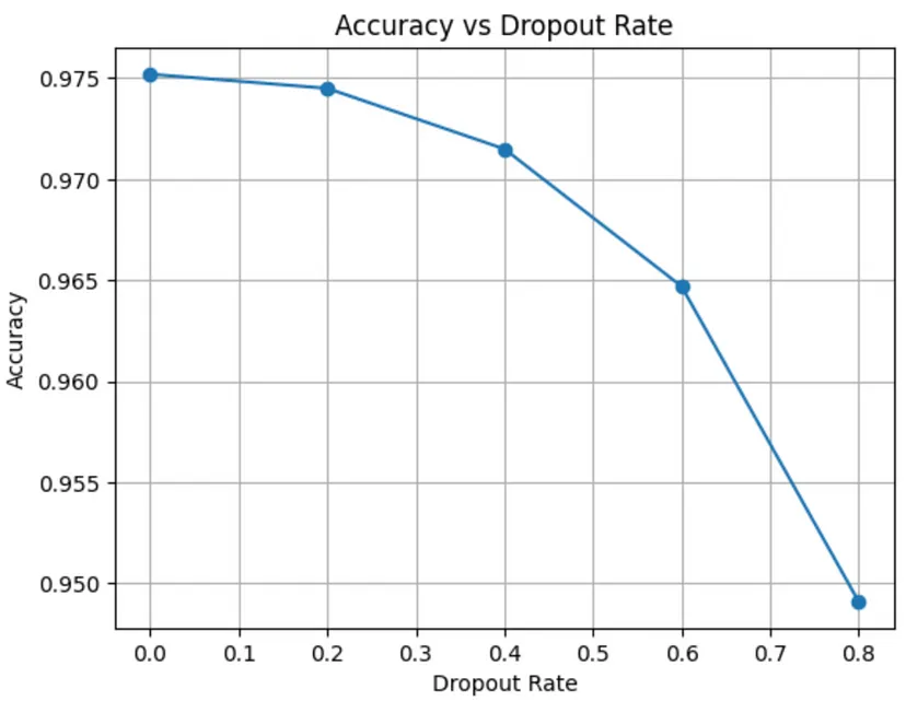
- Even at a rate of 80%, it doesn’t effect the accuracy a great deal, which means that removing excess neurons is certainly an optimization to be considered.
- Example:
- Functional Ablation: Change the activation functions of the neurons to different curves, with different amounts of non-linearity. If a more linear activation is acceptable, then a simpler and cheaper model (e.g. linear/logistic regression) may be feasible.
- Example:
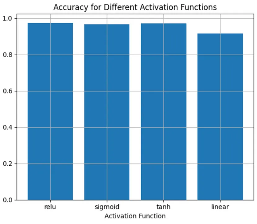
- Non-linearity of some kind is important to this classification task, with “ReLU” and hyperbolic tangent non-linearity being the most effective.
- Example:
- Input Ablation: Remove or alter features and see how it effects the accuracy.
- Includes adding noise (e.g. distorting images) or rotating images, removing a predictor or columns of pixels, removing a transformation.
- Example: Removing columns of pixels for each image
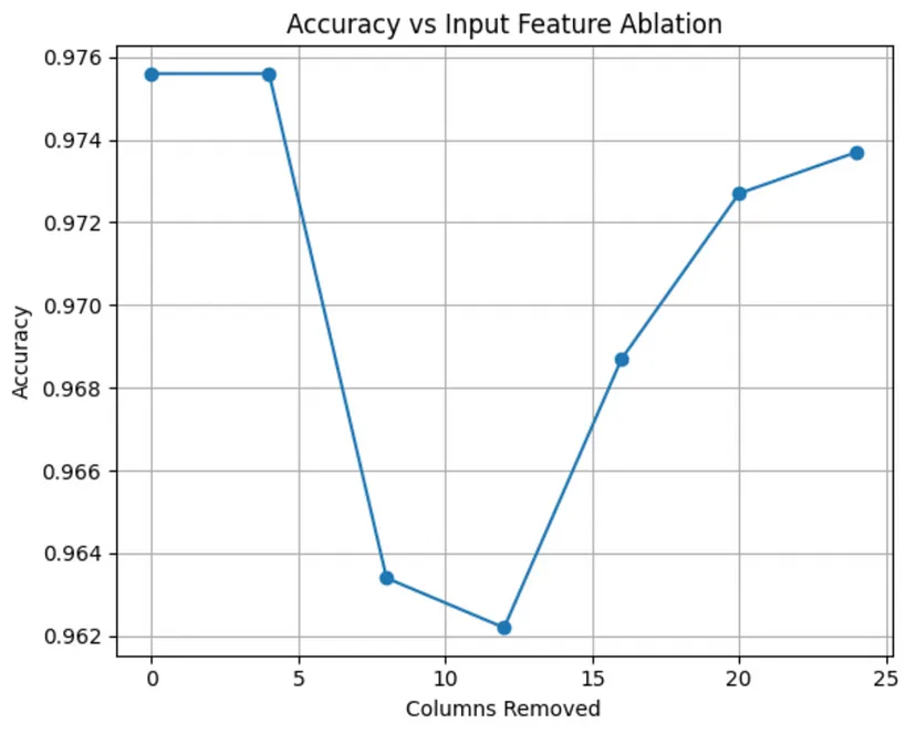
- A slight dip in accuracy when we remove columns 8 to to 12, and a rise again after that. That suggests that on average, the more “sensitive” character geometry lies in those center columns, but the other columns especially close to the beginning and end could potentially be removed for an optimization effect.
- Example: Adding Gaussian noise to distort images
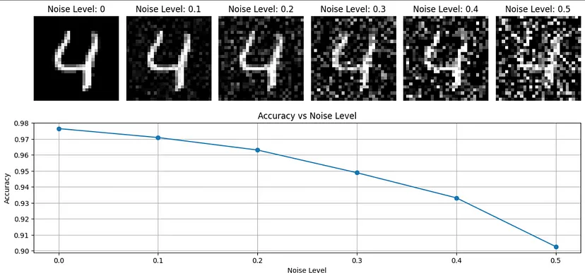
- Distortion has a substantial effect on this model’s accuracy.
- Neuronal Ablation: Remove varying percentages of neurons from our neural network (i.e. dropout rate)
Reinforcement Learning
- Packages
- {multiRL} - Modularizes the Markov Decision Process (MDP) into six core components, enabling users to flexibly construct the Rescorla-Wagner Model for Multi-Armed Bandit tasks
- Involves training a smart agent that can learn to perform a goal through trial & error in an environment and at the end of the training we have an agent that can perform the goal in real life independently
- A type of machine learning problem where, rather than making a single decision, you have to make multiple sequential decisions as part of a strategy
- RL does not require any explicit labels to be provided unlike in supervised learning techniques
- Use Cases
- Email
- What’s the most optimal time for each user as to when they’ll want to read it.
- How many is too many emails per user?
- Dynamic paywall metering
- Help make the decision about a tradeoff between making revenue through serving ads by allowing users to read articles for free and making revenue through subscriptions by blocking free access with a digital paywall (after a certain number of free articles), inducing the user to subscribe
- Email
- Deep Q Network (DQN)
- A combination of the principles of deep learning and Q-learning
- Q-learning is an algorithm of a class of RL solutions called tabular solutions which aims to learn the q-values for each state.
- Q-value of a state is the cumulative (discounted) reward from all the states that the agent could go in the future.
- An elegant solution for problems that have a finite state spaces such as frozen lake problem.
- Q-learning is an algorithm of a class of RL solutions called tabular solutions which aims to learn the q-values for each state.
- For larger state spaces, this Q-learning gets unwieldy and needs to adopt an approximate way of estimating state value and this class of solution is called ‘approximate methods’.
- DQN is the most popular algorithm among the approximate methods.
- In DQN, the deep learning network serves as a function approximation that estimates the value for a given state/action
- The solution design, the algorithm and the setup would be the same for all the use cases, but the configuration of the MDP (Markov Decision Process)— the states spaces, rewards, actions to be taken would vary for each use case.
- Example
- States — The NL opens/clicks pattern for the last (1/2) months.
- Action — 1–24 hours of the day. This could further be reduced to 12 action values with each action representing a 2 hour period when the email could be send.
- Reward — +2 for a NL click, +1 for a NL open, 0 otherwise
- Example
- A combination of the principles of deep learning and Q-learning