5  Experiments, Stepped Wedge Cluster Design

• Stepped Wedge(https://www.rdatagen.net/post/alternatives-to-stepped-wedge-designs/)
  
  

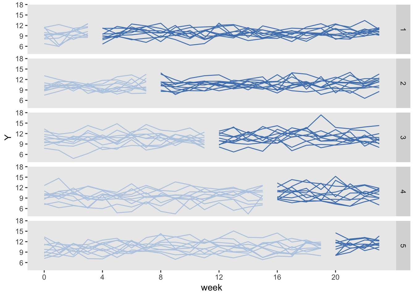
• In the example, the study lasts 24 weeks and is conducted using 50 total sites (geographical locations). Each site will include six patients per week [the “per week” just means each site will have 6 total subjects participating each week as part of control or later in the treatment]. That means if we are collecting data for all sites over the entire study period, we will have 24×6×50=7200 outcome measurements.

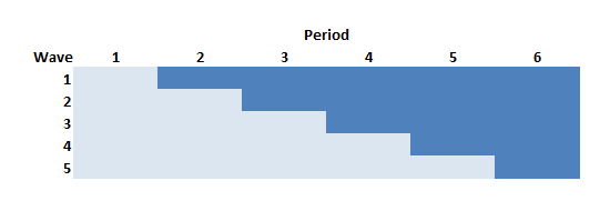
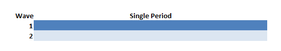
• In the stepped-wedge design, all clusters [I think the clusters are the “waves”] in a trial will receive the intervention at some point, but the start of the intervention will be staggered. The amount of time in each state (control or intervention) will differ for each site (or group of sites if there are waves of more than one site starting up at the same time).

• In this design (and in the others as well) time is divided into discrete data collection/phase-in periods. In the schematic figure, the light blue sections are periods during which the sites are in a control state, and the darker blue are periods during which the sites are in the intervention state. Each period in this case is 4 weeks long.

• Following the Thompson et al. paper, the periods can be characterized as pre-rollout (where no intervention occurs), rollout (where the intervention is introduced over time), and post-rollout (where the all clusters are under intervention). Here, the rollout period includes periods two through five.

• Stepped Wedge with Rollout-Only
  

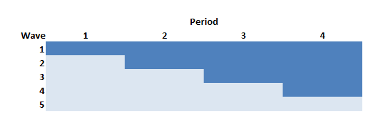
• The Thompson et al. paper argued that if we limit the study to the rollout period only (periods 2 through 5 in the example above) but increase the length of the periods (here, from 4 to 6 weeks), we can actually increase power. In this case, there will be one wave of 10 sites that never receives the intervention.

• The data generation process is exactly the same as above, except the statement defining the length of periods (6 weeks instead of 4 weeks) and starting point (week 0 vs. week 4) is slightly changed

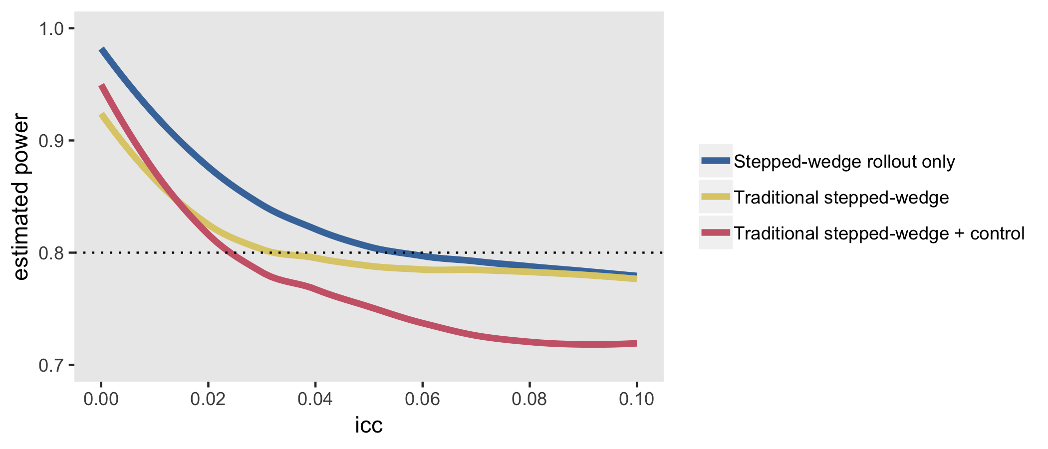
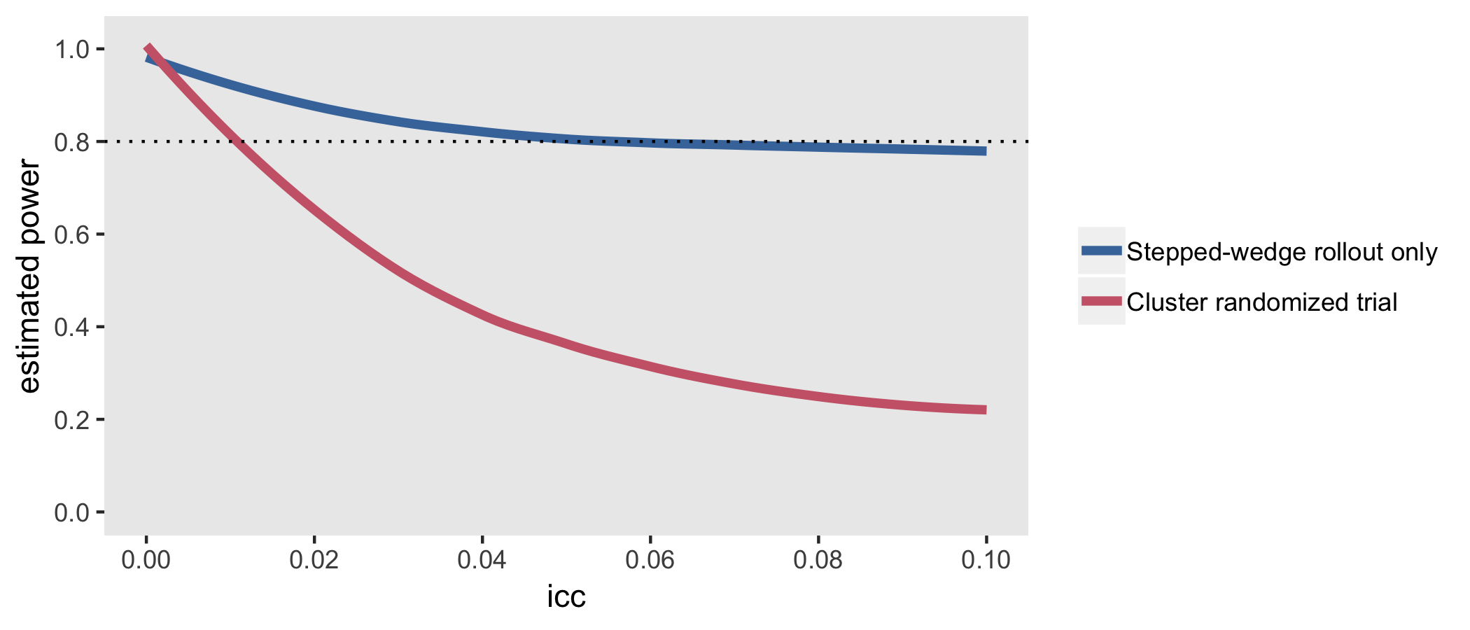
• Stepped wedge with rollout maintains power best as the inter-class correlation (ICC) increases between sites

• 

• Stepped Wedge vs. Cluster Randomized Trial (CRT)
  

  • CRT is a traditional parallel design unlike the stepped design that’s been discussed
  • The simulations confirm findings that the CRT is more efficient than stepped-wedge designs when the ICC is close to zero, but pales in comparison even with ICCs as low as 0.01.

• 

• Intra-cluster correlation (ICC) across time periods

  • (https://www.rdatagen.net/post/intra-cluster-correlations-over-time/)
  • Moving beyond the parallel design (CRT design above) to the stepped-wedge design, time starts to play a very important role. It is important to ensure that we do not confound treatment and time effects; we have to be careful that we do not attribute the_general_changes over time to the intervention. This is accomplished by introducing a time trend into the model. (Actually, it seems more common to include a time-specific effect [dummy vars for each period I assume] so that each time period has its own effect. However, for simulation purposes, I will assume a linear trend.)
  • In the stepped-wedge design, we are essentially estimating within-cluster treatment effects by comparing the cluster with itself pre- and post-intervention. To estimate sample size and precision (or power), it is no longer sufficient to consider a single ICC, because there are now multiple ICC’s - the within-period ICC and the between-period ICC’s. The within-period ICC is what we defined in the parallel design [standard ICC definition in my notebook](since we effectively treated all observations as occurring in the same period.) Now we also need to consider the expected correlation of two individuals in the same cluster in different time periods.
  • If we do not properly account for within-period ICC and the between-period ICC’s in either the planning or analysis stages, we run the risk of generating biased estimates.
  • Side note: according to the standard ICC equation, we can say that correlation between any two subjects in a cluster increases as the variation between clusters increases

• Modeling

  • Traditional parallel clustered design(e.g. CRT above) mixed model
    • (https://www.rdatagen.net/post/intra-cluster-correlations-over-time/)
    • 
    • , where y_ic is a continuous outcome for subject i in cluster c, and X_c is a treatment indicator for cluster c (either 0 or 1). The underlying structural parameters are μ, the grand mean, andβ1, the treatment effect. The unobserved random effects are b_c∼ N(0,σ_b^2), the normally distributed group level effect, and e_ic ∼ N(0, _e^2), the normally distributed individual-level effect. (This is often referred to as the “error” term, but that doesn’t adequately describe what is really unmeasured individual variation.)
  • 
  • Constant (and equal) ICCs over time
    • Assumes that the within-period ICC and between-period ICC’s are equal and constant throughout the study
    • 
    • The key differences between this model compared to the parallel design is the time trend and time-dependent treatment indicator. The time trend accounts for the fact that the outcome may change over time regardless of the intervention. And since the cluster will be in both the control and intervention states we need to have an time-dependent intervention indicator.
    • Within- and between- period ICC is
    • 
    • Between-period ICC means we are estimating the expected correlation between any two subjects i and j in cluster c, one in time period t and the other in time period t’ where (t≠t′). So correlations are being calculated between all pair-wise combinations of the periods. Not just between t and t+1 but also t and t+2, etc.
    • (https://www.rdatagen.net/post/estimating-treatment-effects-and-iccs-for-stepped-wedge-designs/)

library(lme4)
lmerfit <- lmer(Y ~ period + rx + (1| cluster), data = dx)
vars <-as.data.frame(VarCorr(lmerfit))$vcov
iccest <- round(vars[1]/(sum(vars)), 3)

• Different within- and between-period ICCs

  • (https://www.rdatagen.net/post/varying-intra-cluster-correlations-over-time/)

  • Instead of a single cluster level effect, b_c, we have a vector of correlated cluster/time specific effects, b_ct.The vector b_c has a multivariate normal distribution N(0,(σ_b^2)*R).These cluster-specific random effects, (b_c1, b_c2, …, b_cT) [I think T is the number of periods] replace b_c, and the slightly modified data generating model is

  • 

  • How we specify r_0 and r reflects different assumptions about the between-period intra-cluster correlations.

  • (see b_ct distribution specification above)

  • Within-period ICC is still the same

  • 

  • , but the between-period ICC is

• 
  • Case 1: In this first case, the correlation between individuals in the same cluster but different time periods is less than the correlation between individuals in the same cluster and same time period. In other words, ICC_tt != ICC_tt’ [what’s described is actually ICC_tt > ICC_tt’ but that still follows them being “not equal.”]. However the between-period correlation isconstant, or in other words, ICC_tt′ are constant for all t and t′. [So the correlation between individuals within-period is different than between-period but the between-period correlation is the equal for each pair of periods]. We have these correlations when r_0 = ρ and r = 1, such that

library(lme4)
lmerfit <- lmer(Y ~ period + rx + (1| cluster/period) , data = dcs)

The cluster-level period-specific effects are specified in the model as “cluster/period”, which indicates that the period effects are nested within the cluster.

• (https://www.rdatagen.net/post/bayes-model-to-estimate-stepped-wedge-trial-with-non-trivial-icc-structure/)

• Extracting period:cluster variance (σ_w^2), the cluster variance (σ_v^2), and the residual (individual level) variance (σ_e^2) from the model fit allows us to estimate cluster level effects (ρ), the within-period ICC_tt, and the between-period ICC_tt’. Don’t confuse \rho_ρ_ with the ICC. \rho_ρ_ is the correlation between the cluster-level period-specific random effects.

• 

- vs <- as.data.table(VarCorr(lmerfit))$vcov
- rho <- vs[2]/sum(vs[1:2])

• The within-period ICC is the ratio of total cluster variance relative to total variance

• 

iccw <- sum(vs[1:2])/sum(vs

• The between-period ICC_tt’ is really just the within-period ICC_tt adjusted by ρ
• 
• (the result of ICC_tt * ρ)

iccb <- vs[2]/sum(vs)

• Case 2: The correlation between individuals in the same cluster degrades over time [the change from case 1 istime-varying, between-period correlation. ICC_tt remains not equal to ICC_tt’]. Here, the correlation between two individuals in adjacent time periods is stronger than the correlation between individuals in periods further apart. That is ICC_tt’ > ICC_tt’’ if |t’ - t| < |t’’ - t|. This structure can be created by setting r_0 = 1 and r = ρ,

• Last article linked also models this case using {rstan}