Time Series

Misc

Also see EDA, Time Series >> Association
{tseriesEntropy} - Implements an Entropy measure of dependence based on the Bhattacharya-Hellinger-Matusita distance.
- Srho.test - Entropy Test For Serial And Cross Dependence For Categorical Sequences
- Srho.ts - Entropy based measure of serial and cross dependence for continuous data. Implements a normalized version of the Hellinger/Matusita distance

Cross-Correlation Function (CCF)

The correlation between two stationary series. The cross-correlation function (CCF) helps you determine which lags of time series $X$ predicts the value of time series $Y$.
For a set of sample correlations between $x_{t+h}$ and $y_t$ for $h = 0, \pm1, \pm2, \pm3, \ldots$, a negative value for $h$ is a correlation between $x$ at a time before $t$ (i.e. lag) and $y$ at time $t$.
- For instance, consider $h = −2$. The CCF value would give the correlation between $x_{t−2}$ and $y_t$.
Misc
- Packages
  - {ebtools::prewhitened_ccf}
  - {forecast::ggCcf} - You have to manually prewhiten series before using this function.
  - {feasts::CCF} - You have to manually prewhiten series before using this function. Data needs to be a tsibble.
- When calculating correlations between lags of a variable and the variable itself (ACF) or another variable (CCF) you can NOT simply take corr(x_t-k, y_t) for the correlation of x at lag k and y and repeat for all the lags of x.
  - The correlation formula/function requires the mean of the series, you would be using a different mean for x_k for each calculation of the correlation of each pair. The assumption is that the series are (second-order?) stationary and therefore have a constant mean (i.e. each series has 1 mean (and variance)), so the mean(s) of (each) original series should be used in the calculations of the correlations.
  - Source: Modern Applied Statistics with S, Venables and Ripley
  - Compared one against the other in COVID-19 CFR project and they actually produce similar patterns but different values of the CCF. The simple correlation method produced inflated CCF values.
Terms
- Input and Output Series - In a cross-correlation in which the direction of influence between two time-series is hypothesized or known,
  - The influential time-series is called the “input” time-series
  - The affected time-series is called the “output” time-series.
- Lead - When one or more $x_{t+h}$ , with $h$ negative, are predictors of $y_t$, it is sometimes said that x leads y.
- Lag - When one or more $x_{t+h}$, with $h$ positive, are predictors of $y_t$, it is sometimes said that x lags y.
Prewhitening
- If either series contain autocorrelation, or the two series share common trends, it is difficult for the CCF to identify meaningful relationships between the two time series. Pre-whitening solves this problem by removing the autocorrelation and trends.
- Helps to avoid spurious correlations
  - Make sure there’s a theoretical reason for the two series to be related
  - Autocorrelation of at least one series should be removed (transformed to white noise)
    - With autocorrelation present:
      - The variance of cross-correlation coefficient is high and therefore spurious correlations are likely
      - Significance calculations are no longer valid since the CCF distribution will not be normal and the variance is no longer 1/n
  - A problem even with stationary series (even more so with non-stationary series)
  - We expect about 1.75 false alarms out of the 35 sample cross-correlations even after prewhitening
Steps
1. Test for stationarity
2. Find number of differences to make the series stationary
  - Not sure if each series should be differenced the same number of times
    - Why would you test a seasonal series and non-seasonal series for an association?
    - The requirement is stationarity, so maybe try using the highest difference needed between both series
      - In dynamic regression, Hyndman says difference all variables if one needs differencing, so proabably applicable here.
  - Some examples also used log transformation , but when I did, it produced nonsensical CCF values. (covid cfr project). So, beware.
3. Seasonal Difference before differencing for trend
4. (Optional) Create lag scatter plots of the differenced series and look for patterns to get an idea of the strength of the linear correlation (See EDA, Time Series >> Association)
  - If there’s a nonlinear pattern, might be difficult or might not to use a nonlinear or nonparametric correlation function. See 3rd bullet under CCF header above for discussion of stationarity assumption. May not be necessary with another correlation type.
5. Prewhiten both series (cryer, chan method)
6. Apply correlation function

Example COVID-19 CFR project

# Number of differences
ind_cases_diff <- forecast::ndiffs(ind_cases_ts)
ind_deaths_diff <- forecast::ndiffs(ind_deaths_ts)
# Number of seasonal differences
ind_cases_sdiff <- forecast::nsdiffs(ind_cases_ts)
ind_deaths_sdiff <- forecast::nsdiffs(ind_deaths_ts)
# Only detrending differences; No seasonal diffs needed
ind_cases_proc <- diff(ind_cases_ts, ind_cases_diff)
ind_deaths_proc <- diff(ind_deaths_ts, ind_deaths_diff)

# Fit AR model with processed input series
ind_cases_ar <- ind_cases_proc %>%
  ts_tsibble() %>%
  model(AR(value ~ order(p = 1:30), ic = "aicc"))
# Pull AR coefs
ind_ar <- coef(ind_cases_ar) %>% 
  filter(stringr::str_detect(term, "ar")) %>% 
  pull(estimate)
# Linearly filter both input and output series using coefs
ind_cases_fil <- 
  stats::filter(ind_cases_proc, 
                filter = c(1, -ind_ar),
                method = 'convolution', 
                sides = 1)
ind_deaths_fil <- 
  stats::filter(ind_deaths_proc, 
                filter = c(1, -ind_ar),
                method = 'convolution', 
                sides = 1)
# spike at -20 with corr = 0.26; nonsensical lags at -4 and -15, -68
ggCcf(ind_cases_fil, ind_deaths_fil)

Distances

The smaller the total distance between two series, the greater the association.
Distance algorithms in the {dtw} and {dtwclust} packages
Other packages
- {distantia} - Qantifies dissimilarity between multivariate ecological time-series (METS)
- {IncDTW} - Fast DTW in C++; Incremental Calculation of Dynamic Time Warping
  - Incremental calculation of DTW (reduces runtime complexity to a linear level for updating the DTW distance)
  - Vector-based implementation of DTW which is faster because no matrices are allocated (reduces the space complexity from a quadratic to a linear level in the number of observations)
  - Subsequence matching algorithm runDTW efficiently finds the k-NN to a query pattern in a long time series
Also see Clustering, Time Series >> {dtwclust}

Dynamic Time Warping Distance (DTW)

dtw_basic , dtw2
The distance between 2 series is measured by “warping” the time axis to bring them as close as possible to each other and measuring the sum of the distances between the points.
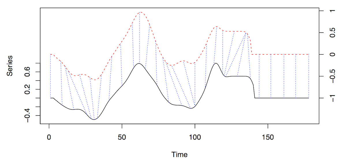
- Figure shows alignment of two series, x and y.
  - The initial and final points of the series must match, but other points along the axis may be “warped” in order to minimize the “cost” (i.e. weighted distance).
  - The dashed blue lines are the warp curves and show how points are mapped to each other.
Hyperparameters:
- Step Pattern - Determines how the algorithm traverses the rows of the LCM to find the optimal path (See Step Patterns Section)
- Window Range - Limits the number lcm calculations for each point (See Window Constraint Section)
Steps
1. Calculate LCM matrix for series X and Y where X is the Query or Test Series and Y is the Reference Series. The LCM is a distance matrix where each element is the distance between the i^th point of series 1 and the j^th point of series 2. (See Local Cost Matrix (LCM) for details)
2. Simultaneously move along each row of the LCM using a chosen step pattern within a chosen window (See Step Patterns and Window Constraints sections to get a visual of this process).
  - The minimum lcm for each point along x-axis is found. The sequence of minimum lcms or minimum alignment is $\phi$ .
  - Calculate the cost, DTW_p, using the LCMs in the minimum alignment
    
    \[ \text{DTW}_p(x, y) = \left(\sum\frac{m_\phi \text{lcm}(k)^p}{M_\phi}\right)^{1/p} \]
    - $m_\phi$: Per-step weighting coefficient (edge weight in patterns fig)
    - $M_\phi$: Normalization constant
    - $k$: Pair of points (or position along the x-axis) in the minimum alignment
  - dtw_basic sets $p = 2$
    - The dtw function in the dtw package doesn’t use p in this equation
3. Choose the alignment with the lowest cost, $\text{DTW}_p$ (i.e. sum of lcm distances for that alignment)

Local Cost Matrix (LCM)

Computed for each pair of series that are compared
The $L_p$ norm (i.e. distance) between the query series and reference series

\[ \text{lcm}(i, j) = \left(\sum_v | x_i^v - y_j^v|^p\right)^{1/p} \]
- $x_i$ and $y_j$ are elements of the test and reference time series respectively
- $v$ stands for “variable” which is for comparing multivariate series
  - i.e. the $L_p$ norm for each pair of points is summed over all variables in the multivariate series.
- $p$ is the order of the norm used
  - e.g. 1 is Manhattan distance; 2 is Euclidean
  - Choice of $p$ only matters if multivariate series are being used
Each $\text{lcm}(i , j)$ value is an element in the $n \times m$ matrix, $\text{LCM}$ where $1 \lt i \lt n$ and $1 \lt j \lt m$

Step Patterns

Determines how algorithm moves across the rows of the LCM to create alignments (warpings of the time axis)
Each pattern is a set of rules and weights
- The rules are used to create different alignments of the LCM (i.e warping of the time axis)
- The edge weights, $m_\phi$, are used in the DTW calculation
Patterns
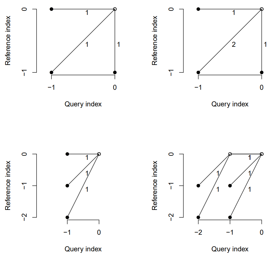
- Patterns in fig
  - Top Row: symmetric1, symmetric2
  - Bottom Row: asymmetric, rabinerJuangStepPattern(4, “c”, TRUE)
    - i.e. Rabiner-Juang’s type IV with slope weighting
- Only some of the patterns are normalizable (i.e. $M_\phi$ is used in the DTW equation) (normalize argument)
  - Normalization may be important when
    1. Comparing alignments between time series of different lengths, to decide the best match (e.g., for classification)
    2. When performing partial matches (?)
  - For dtw_basic, doc says only supported with symmetric2
  - rabinerJuangStepPattern with slope weighting types c and d are normalizable
  - symmetricP* (where * is a number) are all normalizable (not shown in fig)
- Symmetric (i.e. dist from A to B equals the distance from B to A) only if:
  - Either symmetric1 or symmetric2 step patterns are used
  - Series are equal length after any constraints are used
  - Some Cluster Validity Indicies (CVI) (See Clustering, Time Series >> Cluster Validity Indicies) require symmetric distance functions
- {dtwclust} author says symmetric1 most commonly used. dtw::dtw_basic uses symmetric2 by default.

Window Constraints

Limits the region that the lcm calculation takes place.
- Reduces computation time but makes sense that you don’t want to compare points that are separated by to large a time interval
Sakoe-Chiba window creates a calculation region along the diagonal (yellow blocks) of the LCM
- 1 set of lcm calculations occurs within the horizontal, rectangular block of the query series and the vertical, rectangular block of the reference series.
- Therefore, pairs are chosen in relatively small neighbors around the i^th point of series 1 and the i^th point of series 2, and the window size is size of the neighborhood.
- Sakoe-Chiba requires equal length series, but a “slanted band” is equivalent and works for unequal length series.
  - “Slanted Band” is what’s used by dtwclust when the window constraint is used.
Optimal window size needs to be tuned
- Can marginally speed up the DTW calculation, but they are mainly used to avoid pathological warping
- $w$, the window size, is around half the size of the actual region covered
  - $[(i, j - w), (i, j + w)]$ which has $2w + 1$ elements
- A common w is 10% of the sample size, smaller sizes sometimes produce better results

Lower Bounds (LB)

dtw_lb
Uses a lower bound the dtw distance to speed up computation
- A considerably large dataset would be needed before the overhead of DTW becomes much larger than that of dtw_lb’s iterations
- May only be useful if one is only interested in nearest neighbors, which is usually the case in partitional clustering
Steps
1. Calculates an initial estimate of a distance matrix between two sets of time series using lb_improved
  - Involves the “lower bound” calculation (Didn’t get into it)
2. Uses the estimate to calculate the corresponding true DTW distance between only the nearest neighbors (row-wise minima of dist.matrix) of each series in $x$ found in $y
3. Updates distance matrix with DTW values
4. Continues iteratively until no changes in the nearest neighbors occur
Only if dataset is very large will this method will be faster than dtw_basic in the calculation of DTW
Not symmetric, no multivariate series
Requires
- Both series to be equal length
- Window constraint defined
- Norm defined
Value of LB (tightness of envelope around series) affected by step pattern which is set in dtw_basic and included via … in dtw_lb
- Size of envelopes in general: LB_Keoghp < LB_Improvedp < DTWp

Soft DTW

sdtw
“Regularizes DTW by smoothing it” (¯\_(ツ)_/¯)
- “smoothness” controlled by gamma
  - Default: 0.01
  - With lower values resulting in less smoothing
Uses a gradient to efficiently calculate cluster prototypes
Not recommended for stand-alone distance calculations
- Negative values can happen
Symmetric and handles series of different lengths and multivariate series

Shape-based Distance (SBD)

\[ \text{SBD} (x,y) = 1-\frac{\max{\text{NCC}_c (x,y)}}{\lVert x \rVert_2 \lVert y \rVert_2} \]

SBD
Used in k-Shape Clustering
- Based on the cross-correlation with coefficient normalization (NCCc) sequence between two series
Fast (uses FFT to calc), competitive with other distance algorithms, and supports series with different lengths
Symmetric, no multivariate series
In preprocessing argument, set to z-normalization

Triangular Global Alignment Kernel Distance

\[ \begin{aligned} &\text{TGAK}(x,y,\sigma,T) = \frac{\omega(i,j)\kappa(x,y)}{2-\omega(i,j)\kappa(x,y)} \\ &\begin{aligned} \text{where}\quad &\omega(i,j) = \left(1-\frac{|i-j|}{T}\right)_+ \\ &\kappa(x,y)= e^{-\phi_\sigma(x,y)} \\ &\phi_\sigma(x,y) = \frac{1}{2\sigma^2}\lVert x-y \rVert^2 + \log \left(2-e^{-\frac{\lVert x-y \rVert^2}{2\sigma^2}}\right) \end{aligned} \end{aligned} \]

GAK
“Regularizes DTW by smoothing it” (¯\_(ツ)_/¯)
Symmetric when normalized (dist a to b = dist b to a)
Supports multivariate series and series of different length (as long as one series isn’t half the length of the other)
Slightly more computationally expensive than DTW (… that equation🥴)
- $\sigma$ can defined by the user but if left as NULL, the function estimates it
- $T$ is the triangular constraint and is similar to the window constraint in DTW but there no argument for it, so I guess it’s taken care of
- No idea what $i$ and $j$ refer to since x and y are also used.
  - Would have to look it up in the original paper or there is a separate website and package for it
If normalize = TRUE, then a distance is returned, can be compared with the other distance measure, and used in clustering
- If FALSE, a similarity is returned