Discrete
Misc
- Also see Regression, Other
- Packages
- {glmnet}
- {contingencytables}
- Companion package for the Statistical Analysis of Contingency Tables book
- {brglm2}
- Estimation and inference from generalized linear models using various methods for bias reduction
- Can be used in models with Separation (See Diagnostics, GLM >> Separation)
- Able to fit poisson and negative binomial models
- Reduction of estimation bias is achieved by solving either:
- The mean-bias reducing adjusted score equations in Firth (1993) and Kosmidis & Firth (2009)
- The median-bias reducing adjusted score equations in Kenne et al (2017)
- The direct subtraction of an estimate of the bias of the maximum likelihood estimator from the maximum likelihood estimates as prescribed in Cordeiro and McCullagh (1991).
- {singleRcapture} - Population estimates from count models (includes zero-inflated and 1-inflated distributions
- {PLNmodels} - Poisson Lognormal Models
- Analyze multivariate count data with the Poisson log-normal model
- {sdlrm} - Modified Skew Discrete Laplace Regression for Integer-Valued and Paired Discrete Data
- Most useful for the analysis of integer-valued data and experimental studies in which paired discrete observations are collected
- Resources
- Discrete Analysis Notebook - Notes from Agresti books and PSU Course
- Statistical Analysis of Contingency Tables (R >> Documents >> Regression)
- Covers effect size estimation, confidence intervals, and hypothesis tests for the binomial and the multinomial distributions, unpaired and paired 2x2 tables, rxc tables, ordered rx2 and 2xc tables, paired cxc tables, and stratified tables.
- Econometric Analysis of Cross-Section and Panel Data - Wooldridge (R >> Documents >> Econometrics), Ch.19
- Also see this Thread and Stack Exchange Post
- The post argues that Negative Binomial (NB) models should almost never be used and cites the Wooldridge book. Just skimming the chapter on NB models, Wooldridge talks a lot about how in many cases the Poisson model is more efficient that the NB model, but I need to read in more detail about coefficient bias. He provides guidelines by referring to assumptions earlier in the chapter, and I didn’t read those.
- In the thread, he says if there’s overdispersion present, you should just use Poisson with Robust Standard Errors.
- He says for interpreting the coefficients of an NB model to be valid, the conditional distribution (i.e. predicted values) must be NB while this isn’t a requirement for the Poisson.
- He does concede for prediction, there aren’t concerns about using a NB
- For Diagnostics see:
- {DHARMa} - Built for Mixed Effects Models for count distributions but handles lm, glm (poisson) and MASS::glm.nb (neg.bin)
- Diagnostics, Probabilistic >> Visual Inspection >> Visual Inspection
- Diagnostics, GLM
- With aggregated counts that are bound within a certain range, it can be better to turn the range of counts into percentages (see example) and model those as your outcome
- Distributions
Zero-One Inflated Beta
mod_zoib <-
  brm(bf(outcome_pct ~ 1),
      data = example_data,
      family = zero_one_inflated_beta(),
      cores = 4)
pp_check(mod_zoib)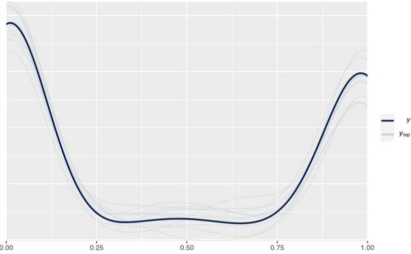
Zero-One Inflated Binomial
- In general, you can have a zero-N inflated binomial
- Example: Aggregated counts from 1 to 32 (Thread)
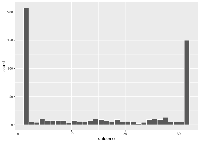
- If something specific is generating 1 and 32 counts
- Ideally you’d do this, but these require creating bespoke distribution families which is possible in STAN
- If you cannot get zero, then a 0-31-inflated binomial works fine.
- If 0 is possible but it didn’t happen, then do a 1-32-inflated binomial.
- More conveniently, you’d transform the range (1-32) to percentages where 100% = 32, and use zero-one inflated beta (currently available in {brms} or zero-one inflated binomial
- Ideally you’d do this, but these require creating bespoke distribution families which is possible in STAN
- If there is NOT something specific generating the 1 and 32 counts(?)
- You can keep the counts and treat them as an ordered factor
Collapse the counts from 2-31 into a category, so you have 3 categories: 1, 2-31, 32.
Model as an ordered logit
mod_ologit <-
  brm(bf(outcome_factor ~ 1),
      data = example_data,
      family = cumulative,
      cores = 4)
pp_check(mod_ologit)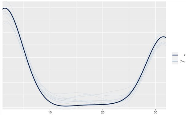
- You can keep the counts and treat them as an ordered factor
- If something specific is generating 1 and 32 counts
- Distributions
Terms
A saturated model is a regression model that includes a discrete (indicator) variable for each set of values the explanatory variables can take.
- Another case is when there are as many estimated parameters as data points.
- e.g. if you have 6 data points and fit a 5th-order polynomial to the data, you would have a saturated model (one parameter for each of the 5 powers of your independant variable plus one for the constant term).
- Multi-variable models require interactions to be able to cover each set of values that the explanatory variables can take (see 3rd example)
- Since saturated models, perfectly model the sample, they don’t generalize to the population well.
- No data left to estimate variance.
- Examples of Saturated Models
Wages ~ College Graduation (binary)
\[ \operatorname{Wages}_i = \alpha + \beta \:\mathbb{I}\{\operatorname{College Graduate}\}_i + \epsilon_i \]
Wages ~ Schooling (discrete, yrs).
\[ \begin{align} \operatorname{Wages} &= \alpha + \beta_1 \:\mathbb{I}\{s_i = 1\} + \beta_2 \:\mathbb{I}\{s_i = 2\} + ⋯ + \beta_T \:\mathbb{I}\{s_i = T\} &\text{where}\quad s_i \in \{0, 1, 2,...T\} \end{align} \]
- 0 is the reference level; \(\beta\) is the effect of j years of schooling.
Wages ~ College Graduation + Gender + Interaction.
\[ \operatorname{Wages} = \alpha + \beta_1 \:\mathbb{I}{\operatorname{College Graduate}} + \beta_2 \:\mathbb{I}\{\operatorname{Female}\} + \beta_3 \:\mathbb{I}\{\operatorname{College Graduate}\} \times \:\mathbb{I}\{\operatorname{Female}\} + ε \]
- \(\mathbb{E}[\operatorname{Wages}_i | \operatorname{College Graduate}_i = 0, \operatorname{Female}_i = 0] = \alpha\)
- Expected value of Wages for individual i given they’re not a college graduate and are male
- \(\mathbb{E}[\operatorname{Wages}_i | \operatorname{College Graduate}_i = 1, \operatorname{Female}_i = 0] = \alpha + \beta_1\)
- \(\mathbb{E}[\operatorname{Wages}_i | \operatorname{College Graduate}_i = 0, \operatorname{Female}_i = 1] = \alpha + \beta_2\)
- \(\mathbb{E}[\operatorname{Wages}_i | \operatorname{College Graduate}_i = 1, \operatorname{Female}_i = 1] = \alpha + \beta_1 + \beta_2 + \beta_3\)
- \(\mathbb{E}[\operatorname{Wages}_i | \operatorname{College Graduate}_i = 0, \operatorname{Female}_i = 0] = \alpha\)
- Another case is when there are as many estimated parameters as data points.
Null Model has only one parameter, which is the intercept.
- This is essentially the mean of all the data points.
- For a bivariate model, this is a horizontal line with the same prediction for every point
Deviance
\[ D = 2(L_S - L_P) = 2(\operatorname{loglik}(y\;|\;y) - \operatorname{loglik}(\mu\;|\;y)) \]
- \(L_S\) is the saturated model
- \(L_P\) is the “proposed model” (i.e. the model being fit)
Binomial
Packages
{fbglm} (Paper) - Fits a fractional binomial regression model to count data with excess zeros using maximum likelihood estimation
- Also see Distributions >> Misc for the {frbinom} package to generation random variables, etc.
- Currently not suitable (i.e. computationally expensive) for a large data set since the distribution’s pmf doesn’t have a closed form solution.
Example: UCB Admissions
# Array to tibble (see below for deaggregation this to 1/0)
ucb <-
    as_tibble(UCBAdmissions) %>%
    mutate(across(where(is.character), ~ as.factor(.))) %>%
    pivot_wider(
        id_cols = c(Gender, Dept),
        names_from = Admit,
        values_from = n,
        values_fill = 0L
      )

## # A tibble: 12 × 4
##    Gender Dept     Admitted Rejected
##    <fct>  <fct>      <dbl>    <dbl>
##  1 Male      A          512      313
##  2 Female    A           89       19
##  3 Male      B          353      207
##  4 Female    B           17        8
##  5 Male      C          120      205
##  6 Female    C          202      391
##  7 Male      D          138      279
##  8 Female    D          131      244
##  9 Male      E           53      138
## 10 Female    E           94      299
## 11 Male      F           22      351
## 12 Female    F           24      317

glm(
  cbind(Rejected, Admitted) ~ Gender + Dept,
  data = ucb,
  family = binomial
)
## Coefficients:
## (Intercept)  GenderMale        DeptB        DeptC        DeptD        DeptE
##    -0.68192     0.09987      0.04340      1.26260      1.29461      1.73931
##      DeptF
##    3.30648
##
## Degrees of Freedom: 11 Total (i.e. Null);  5 Residual
## Null Deviance:     877.1
## Residual Deviance: 20.2 AIC: 103.1
cbind(Rejected, Admitted)says that “Rejected” is the response variable since it is listed first in thecbindfunction- Can also use a logistic model, but need case-level data (e.g. 0/1)
Deaggregate count data into 0/1 case-level data
data(UCBadmit, package = "rethinking")
ucb <- UCBadmit %>%
  mutate(applicant.gender = relevel(applicant.gender, ref = "male"))

# deaggregate to 1/0
deagg_ucb <- function(x, y) {
  UCBadmit %>%
    select(-applications) %>%
    group_by(dept, applicant.gender) %>%
    tidyr::uncount(weights = !!sym(x)) %>%
    mutate(admitted = y) %>%
    select(dept, gender = applicant.gender, admitted)
}
ucb_01 <- purrr::map2_dfr(c("admit", "reject"),
                          c(1, 0),
                          ~ disagg_ucb(.x, .y)
)
Example: Treatment/Control
Disease No Disease Treatment 55 67 Control 42 34 df <- tibble(treatment_status = c("treatment", "no_treatment"), disease = c(55, 42), no_disease = c(67,34)) %>% mutate(total = no_disease + disease, proportion_disease = disease / total) model_weighted <- glm(proportion_disease ~ treatment_status, data = df, family = binomial, weights = total) model_cbinded <- glm(cbind(disease, no_disease) ~ treatment_status, data = df, family = binomial) # Aggregated counts expanded into case-level data df_expanded <- tibble(disease_status = c(1, 1, 0, 0), treatment_status = rep(c("treatment", "control"), 2)) %>% .[c(rep(1, 55), rep(2, 42), rep(3, 67), rep(4, 34)), ] # logistic model_expanded <- glm(disease_status ~ treatment_status, data = df_expanded, family = binomial("logit"))- All methods are equivalent
- “disease” is listed first in the
cbindfunction, therefore it is the response variable.
Poisson
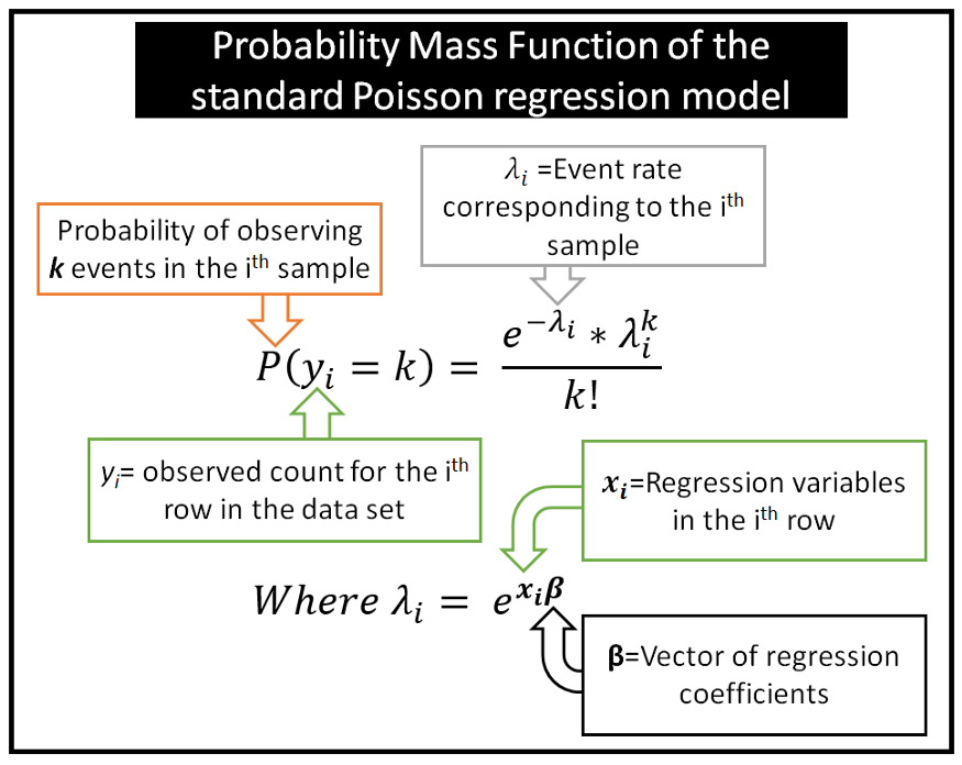
- Misc
- Overdispersion is when the sample variance is greater than the assumed variance which \(\text{var}(y) = \mu\).
- Dispersion, \(\phi = \frac{\text{var}(y)}{\mu}\)
- Significance Test:
AER::dispersiontest(glm_fit)- p-value < 0.05 indicates that significant overdispersion is present.
- Solutions
- Quasi-Poisson which adjusts the S.E. and t-stats: \(\phi= \frac{\chi^2}{(N-p)}\)
- \(\chi^2\) is chi-square; \(N\) is the sample size; \(p\) is the number of model parameters
- family = “quasi-poisson” or “quasipoisson”
- Robust Standard Errors:
- Negative Binomial
- {spdep::EBlocal} (Vignette) - Geospatial; Computes local empirical Bayes estimates that shrinks location rates towards a neighborhood mean
- Acts as a counts smoother for locations with high variance and small populations. Should help with outliers and overdispersion.
- If there are many zero counts, some estimates may be affected by division by zero
- Might also be useful as a preprocessing step.
- Quasi-Poisson which adjusts the S.E. and t-stats: \(\phi= \frac{\chi^2}{(N-p)}\)
- Using an Identity Link
- If the true relationship is additive (e.g., a treatment increases cases by a fixed amount rather than a percentage), the identity link is more appropriate.
- The identity link constrains predictions to remain linear, which may be more realistic in some cases.
- Issues
- \(\mu\) must be positive, but the linear predictor can yield negative values, which leads to nonsensical predictions.
- The model may fail to converge if the optimization encounters negative means
- Solutions
- Use starting values (See Regression, Logistic >> Starting Values)
- {glm2} (Vignette) - Fits models with a modified default fitting method that provides greater stability for models that may fail to converge using glm
- Sometimes the method (step-halving) that glm uses when it fails to converge doesn’t get activated. This package uses that method at the start.
- Could still require starting values.
- Bayesian Methods
- Overdispersion is when the sample variance is greater than the assumed variance which \(\text{var}(y) = \mu\).
- Assumptions
- The mean is equal to the variance
- The outcome is an integer
- Events are independent (e.g. scoring a goal doesn’t impact the scoring of another goal)
- Time period (or space) is fixed
- Homogeneity (e.g. each team has the same probability of scoring a goal)
- Easily violated
- Violations leads to overdispersion
- Multiple events do not happen at the same time (or space)
- Or the distribution is actually Binomial and n is sufficiently larger than “successes.”
- Can lead to negative predictions
- Interpretation
Effect of a binary treatment
\[ e^\beta = \mathbb{E}[Y(1)/\mathbb{E}Y(0)] = \theta_{\text{ATE%}} + 1 \]
- \(\theta\) is the effect interpreted as a percentage
- \(\mathbb{E}[Y(1)]\) is the expected value of the outcome for a subject assigned to Treatment.
- Therefore, \(e^\beta - 1\) is the average percent increase or decrease from baseline to treatment
- Parameter may difficult to interpret in contexts where Y spans several order of magnitudes.
- Example: The econometrician may perceive a change in income from $5,000 to $6,000 very differently from a change in income from $100,000 to $101,000, yet both those changes are treatment effects in levels of $1,000 and thus contribute equally to θATE%.