Logistic
Misc
- Also see
- Packages
- {glmnet}
- {brglm2}
- Estimation and inference from generalized linear models using various methods for bias reduction
- Can be used in models with Separation (See Diagnostics, GLM >> Separation)
- Able to fit multinomial and logistic regression models
- Reduction of estimation bias is achieved by solving either:
- The mean-bias reducing adjusted score equations in Firth (1993) and Kosmidis & Firth (2009)
- The median-bias reducing adjusted score equations in Kenne et al (2017)
- The direct subtraction of an estimate of the bias of the maximum likelihood estimator from the maximum likelihood estimates as prescribed in Cordeiro and McCullagh (1991).
- {LogisticCopula} (Paper) - A Copula Based Extension of Logistic Regression that aims to account for non-linear main effects and complex interactions, while keeping the model inherently explainable.
- Uses a generative specification of the model, consisting of a combination of certain margins on natural exponential form, combined with vine copulas.
- The model is constructed by starting from a Naive Bayes model resulting in linear log odds, and then adding vine copula terms which introduce additional non-linear effects and interaction terms in the form of between - covariate dependence, conditional on the response.
- The resulting model for the log odds ratio becomes a sum of the logistic regression model with linear main effects and some non-linear terms that involve two covariates or more.
- Performs best when non-linearities and complex interactions are present, even when n is not large compared to p.
- Uses a generative specification of the model, consisting of a combination of certain margins on natural exponential form, combined with vine copulas.
glmneeds the outcome to be numeric 0/1 (not factor)- Regularized Logistic Regression is most necessary when the number of candidate predictors is large in relationship to the effective sample size 3np(1−p) where p is the proportion of Y=1 Harrell
- Sample size requirements
- Harrell
- These are conservative estimates. Sample size estimates assume an event probability of 0.50.
- For just estimating the intercept and a margin of error for predicted probabilities of 0.1
- With no covariates (i.e. population is homogeneous), n = 96
- With 1 categorical covariate, n = 96 for each level of the covariate
- e.g. For gender, you need 96 males and 96 females
- For just estimating the intercept and a margin of error for predicted probabilities of 0.05
- With no covariates (i.e. population is homogeneous), n = 384
- If true probabilities of event (and non-event) are known to be extreme, i.e. \(p \notin [0.2, 0.8]\), n = 246
- For estimating predicted probabilities with 1 continuous predictor
- For a margin of error of 0.1, n = 150
- For a margin of error of 0.07, n = 300
- When \(n \lt \frac{p}{2}\), there is almost no relationship between true and estimated ORs (Harrell)
- If \(n\) is too low for \(p\), see Harrell’s checklist.
- Papers that study sample size for logistic regression
- Harrell
- “Stable” AUC requirements for 0/1 outcome:
- paper: Modern modelling techniques are data hungry: a simulation study for predicting dichotomous endpoints | BMC Medical Research Methodology | Full Text
- Logistic Regression: 20 to 50 events per predictor variable
- Random Forest and SVM: greater than 200 to 500 events per predictor variable
- Non-Collapsibility: The conditional odds ratio (OR) or hazard ratio (HR) is different from the marginal (unadjusted) ratio even in the complete absence of confounding.
- Don’t use percents to report probabilities (Harrell)
- Examples (Good)
- The chance of stroke went from 0.02 to 0.03
- The chance of stroke increased by 0.01 (or the absolute chance of stroke increased by 0.01)
- The chance of stroke increased by a factor of 1.5
- If 0.02 corresponded to treatment A and 0.03 corresponded to treatment B: treatment A multiplied the risk of stroke by 2/3 in comparison to treatment B.
- Treatment A modified the risk of stroke by a factor of 2/3
- The treatment A: treatment B risk ratio is 2/3 or 0.667.
- Examples (Good)
- RCTs (notes from Harrell)
- outcome ~ treatment
- These simple models are for homogeneous patient populations, i.e., patients with no known risk factors
- When heterogeneity (patients have strong risk factors) is present, patients come from a mixture of distributions and this causes the treatment effect to shrink towards 0 in logistic and cox-ph models. (see Ch. 13 for in Harrell’s biostats book details
- In a linear model, this heterogeneity (i.e. risk factors) that’s unaccounted for gets absorbed into the error term (residual variance ↑, power ↓), but logistic/cox-ph models don’t have residuals so the treatment effect shrinks as a result.
- outcome ~ treatment + risk_factor_vars
- Adjusting for risk factors stops a loss of power but never increases power like it does for linear models.
- In Cox and logistic models there are no residual terms, and unaccounted outcome heterogeneity has nowhere to go. So it goes into the regression coefficients that are in the model, attenuating them towards zero. Failure to adjust for easily accountable outcome heterogeneity in nonlinear models causes a loss of power as a result.
- Modeling is a question of approximating the effects of baseline variables that explain outcome heterogeneity. The better the model the more complete the conditioning and the more accurate the patient-specific effects that are estimated from the model. Omitted covariates or under-fitting strong nonlinear relationships results in effectively conditioning on only part of what one would like to know. This partial conditioning still results in useful estimates, and the estimated treatment effect will be somewhere between a fully correctly adjusted effect and a non-covariate-adjusted effect.
- outcome ~ treatment
Interpretation
Misc
- Also see Visualization >> Log Odds Ratios vs Odds Ratios
- A logit link, which means that the effects (parameter magnitudes or CIs) can’t easily be translated to the probability scale without picking a baseline value (unlike identity-link models or log-link models such as Poisson regression). Consider also reporting the marginal effects as they are more interpretable. See Marginal Effects
- “Divide by 4” shortcut (Gelman)
- Valid for coefficients and standard errors
- “1 unit increase in X results in a β/4 increase in probability that Y = 1”
- Always round down
- Better appproximations when the probability is close to 0.50
Definitions
.png)
Example: Event probability is 0.20 (source)
# odds
o <- 0.2/(1 - 0.2)

# log odds
lo <- log(o)
lo <- qlogis(0.2)

# reconstruct probability
p <- plogis(lo)
p <- o / (1 + o)
Effect is non-linear in p
.png)
Probability prediction:
\[p(x) = \text{logit}^{-1}(a + bx) = \frac{1}{1 + \exp(-a - bx)}\]
Odds Ratio - Describes the percent change in odds of the outcome based on a one unit increase in the input variable.
A ratio of odds. The ratio of something that’s happening to something that’s not happening
Associated with terms like better chances, greater odds
OR significance is being different from 1 and log odds ratios (logits) significance is being different from 0
logit(p) = 0, p = 0.5, OR = 1
logit(p) = 6, p = always (close to 1)
logit(p) = -6, p = never (close to 0)
Guidelines
- OR > 1 means increased occurrence of an event (more likely)
- OR < 1 means decreased occurrence of an event (less likely)
- OR = 1 ↔︎ log OR = 0 ⇒ No difference in odds
- OR < 0.5 or OR > 2 ⇒ Moderate effect
- OR > 4 is pretty strong and unlikely to be explained by unmeasured variables
Code
prostate_model %>% broom::tidy(exp = TRUE) ## term estimate std.error statistic p.value ## <chr> <dbl> <dbl> <dbl> <dbl> ## 1 (Intercept) 0.0318 0.435 -7.93 2.15e-15 ## 2 fam_hx 0.407 0.478 -1.88 6.05e- 2 ## 3 b_gs 3.27 0.219 5.40 6.70e- 8- Exponentiates coefficients to get ORs
- Interpretation: the odds ratio estimate of 0.407 means that for someone with a positive family history (fam_hx) of prostate cancer, the odds of their having a recurrence are 59.3% ((1-0.407) x 100) lower than someone without a family history. Similarly, for each unit increase in the baseline Gleason score (b_gs), the odds of recurrence increase by 227% ((3.27-1) x 100).
Risk Ratio
A ratio of probabilities. A ratio of something that’s happening to everything that could happen
Assoicated with terms like: increased risk, higher likelihood
P-Values between odds ratios and risk ratios will not be the same
- So while you can convert ORs to RRs, the p-value of the OR doesn’t transfer
Log-Binomials which calculate risk ratios as effects (and p-values) often fail to converge for rare events (which is why most medical research uses ORs and Logistic Regression)
ORs and RRs can be close in value for rare events.
- Rule of Thumb: When the prevalence of an event is less than 10%, the odds ratio closely approximates the risk ratio.
See Odds Ratio >> Guidelines for interpretation
- Even though RRs have the same guidelines as ORs, ORs typically have a larger magnitude for a given RR. (e.g. RR = 2 \(\rightarrow\) OR = 3.5, RR = 0.5 \(\rightarrow\) OR = 0.2)
Formula
\[\begin{align*} \text{RR} &= \frac{\text{Risk of Category A}}{\text{Risk of Category A}} \\ &= \frac{\frac{\text{\# of category A that experienced event}}{\text{total \# of category A}}}{\frac{\text{\# of category B that experienced event}}{\text{total \# of category B}}} \end{align*}\]
Relationship between odds and probabilities
\[\begin{align} P &= \frac{\text{odds}}{1 + \text{odds}} \\ Odds &= \frac{P}{1-P} \end{align}\]
Relationship between Risk Ratios and Odds Ratios
\[\begin{align} \text{RR} &= \frac{\text{OR}}{1 - I_0 \cdot (1 - \text{OR})} \\ \text{OR} &= \frac{\text{RR} \cdot (1-I_0)}{1-I_0 \cdot \text{RR}} \end{align}\]
\(I_0\) is the baseline risk in the control group (i.e. reference category; the denominator in the RR calculation)
Example:
\[\text{RR} = \frac{\text{Risk of Females}}{\text{Risk of Males}} = \frac{7/10}{2/10} = 3.5\]
- \(I_0 = 2/10 = 0.20\)
Summary
## glm(formula = recurrence ~ fam_hx + b_gs, family = binomial, ## data = .) ## ## Deviance Residuals: ## Min 1Q Median 3Q Max ## -1.2216 -0.5089 -0.4446 -0.2879 2.5315 ## ## Coefficients: ## Estimate Std. Error z value Pr(>|z|) ## (Intercept) -3.4485 0.4347 -7.932 0.00000000000000215 ## fam_hx -0.8983 0.4785 -1.877 0.0605 ## b_gs 1.1839 0.2193 5.399 0.00000006698872947 ## ## (Intercept) *** ## fam_hx . ## b_gs *** ## --- ## Signif. codes: ## 0 '***' 0.001 '**' 0.01 '*' 0.05 '.' 0.1 ' ' 1 ## ## (Dispersion parameter for binomial family taken to be 1) ## ## Null deviance: 281.88 on 313 degrees of freedom ## Residual deviance: 246.81 on 311 degrees of freedom ## (2 observations deleted due to missingness) ## AIC: 252.81 ## ## Number of Fisher Scoring iterations: 5- The Deviance Residuals should have a Median near zero, and be roughly symmetric around zero. If the median is close to zero, the model is not biased in one direction (the outcome is not over- nor under-estimated).
- The Coefficients estimate how much a change of one unit in each predictor will affect the outcome (in logit units).
- The family history predictor (fam_hx) is not significant, but trends toward an association with a decreased odds of recurrence, while the baseline Gleason score (b_gs) is significant and is associated with an 18% increased log-odds of recurrence for each extra point in the Gleason score.
- Null Deviance and Residual Deviance. The null deviance is measured for the null model, with only an intercept. The residual deviance is measured for your model with predictors. Your residual deviance should be lower than the null deviance.
- You can even measure whether your model is significantly better than the null model by calculating the difference between the Null Deviance and the Residual Deviance. This difference [281.9 - 246.8 = 35.1] has a chi-square distribution. You can look up the value for chi-square with 2 degrees (because you had 2 predictors) of freedom.
- Or you can calculate this in R with
pchisq(q = 35.1, df=2, lower.tail = TRUE)which gives you a p value of 1.
- The degrees of freedom are related to the number of observations, and how many predictors you have used. If you look at the mean value in the prostate dataset for recurrence, it is 0.1708861, which means that 17% of the participants experienced a recurrence of prostate cancer. If you are calculating the mean of 315 of the 316 observations, and you know the overall mean of all 315, you (mathematically) know the value of the last observation - recurrence or not - it has no degrees of freedom. So for 316 observations, you have n-1 or 315, degrees of freedom. For each predictor in your model you ‘use up’ one degree of freedom. The degrees of freedom affect the significance of the test statistic (T, or chi-squared, or F statistic).
- Observations deleted due to missingness - the logistic model will only work on complete cases, so if one of your predictors or the outcome is frequently missing, your effective dataset size will shrink rapidly. You want to know if this is an issue, as this might change which predictors you use (avoid frequently missing ones), or lead you to consider imputation of missing values.
Predicted Risk - predicted probabilities from a logistic regression model that’s used to predict the risk of an event given a set of variables.
str(salespeople) ## 'data.frame': 350 obs. of 4 variables: ## $ promoted : int 0 0 1 0 1 1 0 0 0 0 ... ## $ sales : int 594 446 674 525 657 918 318 364 342 387 ... ## $ customer_rate: num 3.94 4.06 3.83 3.62 4.4 4.54 3.09 4.89 3.74 3 ... ## $ performance : int 2 3 4 2 3 2 3 1 3 3 ... model <- glm(formula = promoted ~ ., data = salespeople, family = "binomial") exp(model$coefficients) %>% round(2) ## (Intercept) sales customer_rate performance2 performance3 ## 0.00 1.04 0.33 1.30 1.98 ## performance4 ## 2.08- Interpretation:
- For two salespeople with the same customer rating and the same performance, each additional thousand dollars in sales increases the odds of promotion by 4%.
- Sales in thousands of dollars
- For two salespeople with the same sales and performance, each additional point in customer rating decreases the odds of promotion by 67%
- Increasing performance4 by 1 unit and holding the rest of the variables constant increases the odds of getting a promotion by 108%.
- I think this is being treated as a factor variable, and therefore the estimate is relative to the reference level (performance1).
- Should be: “Performance4 increases the odds of getting a promotion by 108% relative to having a performance1”
- For two salespeople of the same sales and customer rating, performance rating has no significant effect on the odds of promotion.
- None of the levels of performance were statistically significant
- For two salespeople with the same customer rating and the same performance, each additional thousand dollars in sales increases the odds of promotion by 4%.
- Interpretation:
Assumptions
performance::model_check(mod)- provides a facet panel of diagnostic charts with subtitles to help interprete each chart.- Looks more geared towards a regression model than a logistic model.
- Linear relationship between the logit of the binary outcome and each continuous explanatory variable
car::boxTidwell- May not work with factor response so might need to as.numeric(response) and use 1,2 values instead of 0,1
- p < 0.05 indicates non-linear relationship which is what you want
- Can also look a scatter plot of logit(response) vs numeric predictor
- No outliers
- Cook’s Distance
- Different opinions regarding what cut-off values to use. One standard threshold is 4/N (where N = number of observations), meaning that observations with Cook’s Distance > 4/N are deemed as influential
- Standardized Residuals
- Absolute standardized residual values greater than 3 represent possible extreme outliers
- Cook’s Distance
- Absence of Multicollinearity
- VIF
- Correlation Heatmap
- iid
- Deviance residuals (y-axis) vs row index (x-axis) should show points randomly around zero (y-axis)
- Jesper’s response shows calculation and R code
- I think the dHARMA pkg also handles this
- Deviance residuals (y-axis) vs row index (x-axis) should show points randomly around zero (y-axis)
- Sufficiently large sample size
- Rules of thumb
- 10 observations with the least frequent outcome for each independent variable
- > 500 observations total
- I’m sure Harrell has thoughts on this somewhere
- Rules of thumb
Diagnostics
- Misc
- ** The formulas for the deviances for a logistic regression model are slightly different from other GLMs since the deviance for the saturated logistic regression model is 0 **
- Also see
- Diagnostics, Classification >> Misc >> Workflow
- Diagnostics, GLM
- Brier Score (See Diagnostics, Classification >> Scores)
- Cessie-Houwelingen-Copas-Hosmer Unweighted Sum of Squares Test
- Seems to be more popular than the Cessie-Houwelingen Test below
- Probably due to how popular the Hosmer-Lemeshow test was and the paper he wrote recommending this test instead.
- Packages
- DescTools::HosmerLemeshowTest(model, X)
- X is a matrix (or maybe dataframe) with the covariates of the model and must be specified for the proper test (and not the flawed Hosmer-Lemeshow test)
- Harrellverse:
rms::residuals(rms::lrm(Y ~ X, data = simulated_data, x=TRUE, y=TRUE), type = "gof")
- DescTools::HosmerLemeshowTest(model, X)
- From the example in the {DescTools} docs, p-value < 0.05 indicates a good fit
- Seems to be more popular than the Cessie-Houwelingen Test below
- Cessie-Houwelingen Test
Notes from Introduction to the Cessie-Houwelingen Test Statistic
A comparison of the observed values to the standardized residuals after weighting them by the inverse of the variance of a kernel smoothing function
- The kernel smoothing is particularly important as it accounts for the continuous attributes of covariates, enabling a more detailed and nuanced assessment of how well the model performs
Algorithm
Standardize the Residuals
\[r_i = \frac{Y_i - \pi(X_i)}{\sqrt{\pi(X_i)(1 - \pi(X_i))}}\]
- \(Y_i\) is the observed response
- \(\pi(X_i)\) is the predicted probability
- Dividing by the standard deviation of the predicted probability, \({\sqrt{\pi(X_i)(1 - \pi(X_i))}}\), standardizes the residuals
Apply Kernel Smoothing to the Standardized Residuals
\[\begin{align} &\hat{r}(x) = \sum_{i=1}^n K_h(x - X_i) r_i \\ &\text{where} \;\; K(x) = \begin{cases} \frac{1}{2} & \text{if } |x| \leq 1, \\ 0 & \text{otherwise.} \end{cases} \end{align}\]
- \(K_h\) is the (uniform) kernel function with bandwidth \(h\)
- The bandwidth determines the size of the region over which the residuals are averaged and the kernel function determines the weighting
Calculate the Test Statistic
\[T = n \sum_{i=1}^n \hat{r}(X_i)^2 U(X_i)\]
- \(U(x_i)\) is the inverse of the variance of the smoothed residual at \(X_i\)
- \(n\) is the sample size.
Indicates how much we trust the estimate of the smoothed residual at each observation.
- When squared residuals are weighted by the inverse of their variances, observations with more precise estimates (i.e., lower variance) contribute more to the test statistic, while observations with less precise estimates (i.e., higher variance) contribute less.
Code
Code
leCessie_test <- function(object, bandwidth) { # Define a function to calculate categorical distances categorical <- function(x) { x <- as.matrix(x) retval <- apply(x, 2, function(y) { nrcats <- length(unique(y)) if (nrcats == 1) { disty <- rep(0, length(y) * (length(y) - 1)) } else { disty <- as.numeric(dist(y, 'manhattan') != 0) * nrcats / (nrcats - 1) } return(disty) }) return(rowSums(retval)) } # Store the original object and construct the variable name object.orig <- object Dname <- as.character(object$call$formula) Dname <- paste(Dname[2], Dname[1], Dname[3]) # Arrange variable names in the correct order # Calculate fitted values and residuals from the model fits <- fitted(object) resids <- resid(object, 'response') N <- length(resids) # Extract the model frame and check if response is a matrix obj.frame <- model.frame(object) if (class(obj.frame[[1]]) == 'matrix') stop("Cannot perform test where response is matrix") # Calculate distances for each predictor in the model distances <- lapply(obj.frame[,-1, drop=FALSE], function(x) { if (is.numeric(x)) { scaled_x <- scale(x) dist_x <- as.matrix(dist(scaled_x)) return(0.5 * dist_x * dist_x) # Compute squared Euclidean distance } else if (class(x) == 'factor') { return(categorical(x)) # Use the categorical distance function for factor variables } else { scaled_x <- scale(x[[1]]) dist_x <- as.matrix(dist(scaled_x)) return(0.5 * dist_x * dist_x) # Handle structured variables created from a function } }) # Initialize a matrix for combined distances and fill it dist.mat <- matrix(0, N, N) for (dist_x in distances) { dist.mat[lower.tri(dist.mat)] <- dist.mat[lower.tri(dist.mat)] + sqrt(dist_x[lower.tri(dist_x)]) } dist.mat <- dist.mat + t(dist.mat) # Symmetrize the distance matrix # Set bandwidth if not specified if (missing(bandwidth)) bandwidth <- mean(dist.mat) R.raw <- pmax(1 - dist.mat / bandwidth, 0) # Compute the raw smoother matrix # Calculate smoothed residuals and raw Q smoothres <- t(resids) %*% R.raw Q.raw <- sum(smoothres * resids) # Prepare matrices for the corrected estimation of Q obj.mat <- model.matrix(object.orig) mu2 <- fits * (1 - fits) V <- diag(mu2) Vx <- diag(V) obj.hat <- Vx * obj.mat %*% solve(t(obj.mat) %*% (Vx * obj.mat)) %*% t(obj.mat) R.cor <- (diag(N) - obj.hat) %*% R.raw %*% (diag(N) - obj.hat) # Compute corrected estimated value of Q and its standard error E.Q <- sum(diag(R.cor) * mu2) mu4 <- mu2 * (1 - 3 * mu2) VarQ1 <- sum(diag(R.cor)^2 * (mu4 - 3 * mu2^2)) R.tmp <- R.cor * matrix(rep(mu2, each = N), nrow = N) VarQ2 <- 2 * sum(diag(R.tmp %*% R.tmp)) VarQ <- VarQ1 + VarQ2 # Calculate the test statistic and degrees of freedom Test <- Q.raw * 2 * E.Q / VarQ df <- 2 * E.Q^2 / VarQ # Construct the output output <- data.frame(statistic = Test, df = df, p.value = 1 - pchisq(Test, df), q = Q.raw, e_q = E.Q, se_q = sqrt(VarQ)) return(output) } leCessie_test(glm_model)- Bandwidth is not required but is available for adjustment
Guide: p-value < 0.05 indicates the model does NOT fit the data well
- Given how the p-value is interpreted in the similar test above, might want to double check this from the references in the article or test it out on some sim data (could use that {DescTools} example data)
- Residual Deviance (G2)
- -2 * LogLikelihood(proposed_mod)))
- Null Deviance
- -2 * LogLikelihood(null_mod)))
- i.e. deviance for the intercept-only model
- McFadden’s Pseudo R2 = (LL(null_mod) - LL(proposed_mod)) / LL(null_mod))
See What are Pseudo-R Squareds? for formulas to various alternative R2s for logistic regression
The p-value for this R2 is the same as the p-value for:
- 2 * (LL(proposed_mod) - LL(null_mod))
- Null Deviance - Residual Deviance
- For the dof, use proposed_dof - null_dof
- dof for the null model is 1
- For the dof, use proposed_dof - null_dof
Example: Getting the p-value
m1 <- glm(outcome ~ treat)
m2 <- glm(outcome ~ 1)
(ll_diff <- logLik(m1) - logLik(m2))
## 'log Lik.' 3.724533 (df=3)
1 - pchisq(2*ll_diff, 3)
- Compare nested models
Models
model1 <- glm(TenYearCHD ~ ageCent + currentSmoker + totChol, data = heart_data, family = binomial) model2 <- glm(TenYearCHD ~ ageCent + currentSmoker + totChol + as.factor(education), data = heart_data, family = binomial)- Add Education or not?
Extract Deviances
# Deviances
(dev_model1 <- glance(model1)$deviance)
## [1] 2894.989
(dev_model2 <- glance(model2)$deviance)
## [1] 2887.206
Calculate difference and test significance
# Drop-in-deviance test statistic
(test_stat <- dev_model1 - dev_model2)
## [1] 7.783615

# p-value
1 - pchisq(test_stat, 3)  # 3 = number of new model terms in model2 (i.e. 3(?) levels of education)
## [1] 0.05070196

# Using anova
anova(model1, model2, test = "Chisq")
## Analysis of Deviance Table
##
## Model 1: TenYearCHD ~ ageCent + currentSmoker + totChol
## Model 2: TenYearCHD ~ ageCent + currentSmoker + totChol + as.factor(education)
##  Resid. Df Resid. Dev Df Deviance Pr(>Chi)
## 1      3654    2895.0
## 2      3651    2887.2  3  7.7836  0.0507 .
- |β| > 10
- Extreme
- Implies probabilities close to 0 or 1 which is suspect
- Consider removal of the variable or outlier(s) influencing the model
- Intercepts ≈ -17
- Indicate a need for a simpler model (see bkmk - Troubleshooting glmmTMB)
- If residuals are heteroskedastic, see {glmx}
- neg.bin, hurdle, logistic - Extended techniques for generalized linear models (GLMs), especially for binary responses, including parametric links and heteroskedastic latent variables
- Binned Residuals (unfinished)
It is not useful to plot the raw residuals, so examine binned residual plots
Misc
- {arm} will mask some {tidyverse} functions, so don’t load whole package
Look for :
- Patterns
- Nonlinear trend may be indication that squared term or log transformation of predictor variable required
- If bins have average residuals with large magnitude
- Look at averages of other predictor variables across bins
- Interaction may be required if large magnitude residuals correspond to certain combinations of predictor variables
Process
- Extract raw residuals
- Include
type.residuals = "response"in thebroom::augmentfunction to get the raw residuals
- Include
- Order observations either by the values of the predicted probabilities (or by numeric predictor variable)
- Use the ordered data to create g bins of approximately equal size.
- Default value: g = sqrt(n)
- Calculate average residual value in each bin
- Plot average residuals vs. average predicted probability (or average predictor value)
- Extract raw residuals
Example: vs Predicted Values
arm::binnedplot(x = risk_m_aug$.fitted, y = risk_m_aug$.resid, xlab = "Predicted Probabilities", main = "Binned Residual vs. Predicted Values", col.int = FALSE)Example: vs Predictor
arm::binnedplot(x = risk_m_aug$ageCent,
                y = risk_m_aug$.resid,
                col.int = FALSE,
                xlab = "Age (Mean-Centered)",
                main = "Binned Residual vs. Age")
Check that residuals have mean zero:
mean(resid(mod))Check that residuals for each level of categorical have mean zero
risk_m_aug %>%
  group_by(currentSmoker) %>%
  summarize(mean_resid = mean(.resid))
Marginal Effects
- Misc
- Notes from
- R >> Documents >> Regression >> glm-marginal-effects.pdf
- Also see
- Marginal Effects and Elasticities are similar except elasticities are percent change.
- e.g. a percentage change in a regressor results in this much of a percentage change in the response level probability
- Notes from
- In general
- A “marginal effect” is a measure of the association between an infinitely small change in a regressor and a change in the response variable
- “infinitely small” because we’re using partial derivatives
- Example: If I change the cost (regressor) of taking the bus, how does that change the probability (not odds or log odds) of taking a bus to work instead of a car (response)
- Allows you to ask counterfactuals.
- In OLS regression with no interactions or higher-order term, the estimated slope coefficients are marginal effects, but for glms, the coefficients are not marginal effects at least not on the scale of the response variable
- Marginal effects are partial derivatives of the regression equation with respect to each variable in the model for each unit in the data. (also see notebook, Regression >> logistic section)
- A “marginal effect” is a measure of the association between an infinitely small change in a regressor and a change in the response variable
- Logistic Regression
The partial derivative gives the slope of a tangent line at point on a nonlinear curve (e.g. logit) which is the linear change in probability at a single point on the nonlinear curve
\[\frac {\partial P}{\partial X_{k}} = \beta_{k} \times P \times (1 - P)\]
- Where P is the predicted probability and β is the model coefficient for the kth predictor
- 3 types of marginal effects
- Marginal effect at the Means
- The marginal effect that is “typical” of the sample
- Each model coefficient is multiplied times their respective independent variables mean and summed along with the intercept.
- This sum is transformed from a logit to a probability, P, is used in the partial derivative equation to calculate the marginal effect
- Interpretation
- continuous: an infinitely small change in
while all other predictors are held at their means results in a change in - e.g. an infinitely small change in this predictor for a hypothetical average person results in this amount of change in the dependent variable
- continuous: an infinitely small change in
- “at the medians” can be easily calculated using
marginaleffects::typical(this is outdated) without any columns specified and then used to calculate marginal effects- to get “at the means” you’d have to supply each column with its mean value
- Marginal effect at Representative (“Typical”) Values
- The marginal effect that is “typical” of a group represented in the sample
- A real “average” person doesn’t usually have the mean/median values for predictor values (e.g mean age of 54.68 years), so you might want to find the marginal effect for a “typical” person of a certain demographic or group you’re interested in by specifying values for predictors
- Interpretation
- continuous: an infinitely small change in
for a person with results in a change in
- continuous: an infinitely small change in
- Calculate using
marginaleffects::typical(this is outdated) to specify column values (this is outdated)
- Average Marginal Effect (AME)
- The marginal effect of a case chosen at random from the sample
- Considered the best summary of an independent variable
- Calculate marginal effect for each observation (distribution of marginal effects) and then take the average
- Multiply the model coefficient times each value of an independent variable, repeat for each predictor, sum with intercept, use predicted probabilities to calculate marginal effect, and average all marginal effects across all obseravation for a predictor to get the AME
- Interpretation
- continuous: Holding all covariates constant, an infinitely small change in
results in a change in on average.
- continuous: Holding all covariates constant, an infinitely small change in
- Use
marginaleffects::marginaleffects+summaryortidy
- The marginal effect of a case chosen at random from the sample
- Marginal effect at the Means
- {marginaleffects}
- Example: Palmer penguins data and logistic regression model
Create marginal effects object
mfx <- marginaleffects(mod)
head(mfx)
#>  rowid              term        dydx  std.error large_penguin bill_length_mm
#> 1    1    bill_length_mm 0.017622745 0.007837288            0          39.1
#> 2    1 flipper_length_mm 0.006763748 0.001561740            0          39.1
#> 3    2    bill_length_mm 0.035846649 0.011917159            0          39.5
#> 4    2 flipper_length_mm 0.013758244 0.002880123            0          39.5
#> 5    3    bill_length_mm 0.084433436 0.021119186            0          40.3
#> 6    3 flipper_length_mm 0.032406447 0.008159318            0          40.3
#>  flipper_length_mm species
#> 1              181  Adelie
#> 2              181  Adelie
#> 3              186  Adelie
#> 4              186  Adelie
#> 5              195  Adelie
#> 6              195  Adelie
Average Marginal Effect (AME)
summary(mfx) #> Average marginal effects #> type Term Contrast Effect Std. Error z value #> 1 response bill_length_mm <NA> 0.02757 0.00849 3.24819 #> 2 response flipper_length_mm <NA> 0.01058 0.00332 3.18766 #> 3 response species Chinstrap / Adelie 0.00547 0.00574 -4.96164 #> 4 response species Gentoo / Adelie 2.19156 2.75319 0.62456 #> 5 response species Gentoo / Chinstrap 400.60647 522.34202 4.59627 #> Pr(>|z|) 2.5 % 97.5 % #> 1 0.0011614 0.01093 0.04421 #> 2 0.0014343 0.00408 0.01709 #> 3 2.0906e-06 -0.00578 0.01673 #> 4 0.8066373 -3.20459 7.58770 #> 5 1.2828e-05 -623.16509 1424.37802- Interpretation:
- Holding all covariates constant, for an infinitely small increase in bill length, the probability of being a large penguin increases on average by 2.757%
- Species contrasts are from {emmeans}(also see Post-Hoc Analysis, emmeans)
- Contrasts from get_contrasts.R on package github using
emmeans::contrast(emmeans_obj, method = "revpairwise") - odds ratios
- You can get response means per category on the probability scale using
emmeans::emmeans(mod, "species", type = "response")
- Contrasts from get_contrasts.R on package github using
- Interpretation:
- Other features available for marginaleffects object
tidy- coef stats with AME, similar to summary, just a different a object class I think
glance- model GOF stats
typical- generate artificial predictor values and get marginal effects for them
- median (or mode depending on variable type) values used for columns that aren’t provided
counterfactual- use observed data for all but a one or a few columns. Provide values for those column(s) (e.g. flipper_length_mm = c(160, 180))
- genereates a new larger dataset where each observation has each of the provided values
- Viz
- {modelsummary} tables
plot(error bar plot for AME) andplot_cme(line plot for interaction term)- outputs ggplot objects
- Example: Palmer penguins data and logistic regression model
- Categorical Variables
- The 3 types of marginal effects can be modified for categoricals
- Steps (“at the means”, binary)
- Calculate the predicted probability when the variable = 1 and the other predictors are equal to their means.
- Calculate the predicted probability when the variable = 0 and the other predictors are equal to their means.
- The difference in predicted probabilities is the marginal effect for a change from the “base level” (aka reference category)
- This can extended to categorical variables with multiple categories by calculating the pairwise differences between each category and the reference category (contrasts)
Log Binomial
- Assumes a binomial distribution for a binary outcome but, unlike logistic regression, uses a log link function which automatically gives more interpretable risk ratios as effects.
Misc
- Also see
- Notes from
- Introduction to Regression Methods for Public Health Using R, Ch. 6.21
- Brief introduction with a basic {logbin} example.
- Video: Beyond Logistic Regression: Master Risk Ratios with Log-Binomial by yuzaR
- Introduction to Regression Methods for Public Health Using R, Ch. 6.21
- Packages
glm(..., family = binomial(link = "log"))- Requires you to pick starting values
- Employs step-halving to bring estimates back into the parameter space if the deviance becomes infinite or any fitted values are outside (0, 1) at any iteration. (logbin vignette)
- If a full Fisher scoring step of IRLS (glm fitting method) will lead to either an infinite deviance or predicted values that are invalid for the model being fitted, then the increment in parameter estimates is repeatedly halved until the updated estimates no longer exhibit these features. (glm2 vignette)
- {glm2} (Vignette) - Fits models with a modified default fitting method that provides greater stability for models that may fail to converge using glm
- Sometimes the method (step-halving) that glm uses when it fails to converge doesn’t get activated. This package uses that method at the start.
- Could still require starting values.
- {logbin} (Vignette) - Methods for fitting log-link GLMs and GAMs to binomial data, including EM-type algorithms with more stable convergence properties than standard methods.
- Don’t have to mess with starting values
- Has a variety of methods to aid in convergence and restricting the parameter space so as to keep the predicted probabilities between 0 and 1
- Default: method = “cem” which is a combinatorial EM algorithm
- CEM can be computationally intensive for larger datasets or more complex specifications (e.g. splines).
- Recommended to try using the parameter expanded EM algorithm (method = “em”) and SQUAREM acceleration scheme (acclerate = “squarem”) to speed up convergence .
- Other methods and acceleration schemes are available
- Fits B-splines via
logbin.smooth - Due to the way in which the covariate space is defined in the CEM algorithm, models that include terms that are functionally dependent on one another — such as interactions and polynomials — may give unexpected results. (i.e. interactions and
polyis not supported)- 2-way interactions between factors can be included by calculating a new factor term that has levels corresponding to all possible combinations of the factor levels
- e.g.
heart$AgeSev <- 10 * heart$AgeGroup + heart$Severity - In this example AgeGroup and Severity are each 3-level categorical variables coded as numerics
- Not sure why they multiplied the AgeGroup variable by 10.
- Don’t think marginal effects are possible using this method. If indeed not, then this is not a satisfactory solution. Use glm or glm2.
- Categorical covariates should always be entered directly as factors rather than dummy variables.
- Papers
- Particle swarm optimization with Applications to Maximum Likelihood Estimation and Penalized Negative Binomial Regression
- Uses Partical Swarm optimization via {pyswarm} to fit various mixture models and also Log-Binomial
- Successfully converges where other optimization methods fail. May also be more efficient in some cases.
- Particle swarm optimization with Applications to Maximum Likelihood Estimation and Penalized Negative Binomial Regression
- With logistic regression, the left-hand side is the log of the odds, whereas in log-binomial regression it is the log of the probability (\(p\)).
- Exponentiating a regression coefficient in log-binomial regression results in a Risk Ratio (RR) or Prevalence Ratio (PR).
- A disadvantage of (standard) log-binomial regression is that the left-hand side \(\ln(p)\) is constrained to be positive while the right-hand side can be anything from \(-\infty\) to \(\infty\), and this leads to:
- Convergence issues for extreme data (i.e. rare events which have low prevalence)
- Predicted probabilities > 1 which is nonsensical
Examples
Example 1: Simple Model using a Polynomial and a Spline
pacman::p_load( dplyr, ggplot2, logbin, emmeans, marginaleffects, gtsummary ) theme_set(theme_notebook()) d <- carData::TitanicSurvival |> filter(!is.na(age)) m_poly <- glm(survived ~ poly(age, 3), data = d, family = binomial(link = "log")) m_spl_bin <- logbin.smooth( survived ~ B(age, knot.range = 0:3), data = d )- Both are similar fitting models. {logbin} can’t fit a polynomial, but it can fit a B-spline.
- The polynomial model converges just fine, so no need for starting values or {glm2}
emmeans( m_poly, pairwise ~ age, type = "response", at = list(age = c(quantile(d$age, probs = c(0.05, 0.50, 0.95)))), weights = "prop", infer = TRUE ) # $emmeans # age prob SE df asymp.LCL asymp.UCL null z.ratio p.value # 5 0.558 0.0399 Inf 0.485 0.642 1 -8.154 <.0001 # 28 0.378 0.0181 Inf 0.344 0.415 1 -20.350 <.0001 # 57 0.412 0.0410 Inf 0.339 0.501 1 -8.914 <.0001 # # Confidence level used: 0.95 # Intervals are back-transformed from the log scale # Tests are performed on the log scale # # $contrasts # contrast ratio SE df asymp.LCL asymp.UCL null z.ratio p.value # age5 / age28 1.476 0.124 Inf 1.212 1.8 1 4.632 <.0001 # age5 / age57 1.354 0.165 Inf 1.018 1.8 1 2.489 0.0343 # age28 / age57 0.917 0.104 Inf 0.703 1.2 1 -0.757 0.7293 # # Confidence level used: 0.95 # Conf-level adjustment: tukey method for comparing a family of 3 estimates # Intervals are back-transformed from the log scale # P value adjustment: tukey method for comparing a family of 3 estimates # Tests are performed on the log scale- {emmeans} doesn’t support a logbin.smooth model
- emmeans are the (equally weighted) marginal means and the contrasts are the risk ratios. See the marginal effects tab for interpretation of some of the values.
1avg_comparisons(m_poly) #> Estimate Std. Error z Pr(>|z|) S 2.5 % 97.5 % #> -0.0028 0.00105 -2.66 0.00783 7.0 -0.00486 -0.000736 #> #> Term: age #> Type: response #> Comparison: +1 2avg_predictions(m_poly, variables = list(age = c(5, 28, 57))) #> age Estimate Std. Error z Pr(>|z|) S 2.5 % 97.5 % #> 5 0.558 0.0399 14.0 <0.001 144.9 0.480 0.636 #> 28 0.378 0.0181 20.9 <0.001 320.3 0.343 0.413 #> 57 0.412 0.0410 10.1 <0.001 76.6 0.332 0.492 3slopes(m_poly, variables = "age", newdata = datagrid(age = c(5, 28, 57))) #> age Estimate Std. Error z Pr(>|z|) S 2.5 % 97.5 % #> 5 -0.02563 0.00670 -3.824 <0.001 12.9 -0.03877 -0.01250 #> 28 0.00120 0.00175 0.682 0.495 1.0 -0.00224 0.00463 #> 57 -0.00472 0.00454 -1.039 0.299 1.7 -0.01362 0.00418 #> #> Term: age #> Type: response #> Comparison: dY/dX 4avg_comparisons(m_poly, comparison = "ratioavg", variables = list(age = c(5, 28)) ) #> Estimate Std. Error z Pr(>|z|) S 2.5 % 97.5 % #> 0.678 0.0569 11.9 <0.001 106.1 0.566 0.789 #> #> Term: age #> Type: response #> Comparison: mean(28) / mean(5) 5avg_predictions(m_poly, variables = list(age = c(5, 28, 57)), hypothesis = ratio ~ revpairwise) #> Hypothesis Estimate Std. Error z Pr(>|z|) S 2.5 % 97.5 % #> (5) / (28) 1.476 0.124 11.90 <0.001 106.1 1.233 1.72 #> (5) / (57) 1.354 0.165 8.21 <0.001 52.1 1.031 1.68 #> (28) / (57) 0.917 0.104 8.79 <0.001 59.2 0.713 1.12- 1
- The average effect of increasing the age by 1 unit on the predicted probability of survival.
- 2
- These are the marginal means. The median age, 28, has a survival probability of 37.8% on average.
- 3
- These are the marginel effects (aka simple slopes). At age = 5, the slope is negative which indicates that an increase in age is associated with an decrease in the probability of survival. This changes by age 28 when a slightly positive slope indicates increasing age increases the probability of survival. For ages 28 and 57, the slopes are near zero which indicates a weak assoication with survival. The high p-values suggest this association could be null.
- 4
- One contrast can be calculated with this method. The variables argument only allows for 2 values for a numeric variable contrast.
- 5
- This method calculates all the risk ratios. By using revpairwise, we can replicate the output of {emmeans}. Survival for a person at age 5 is about 1.5 times (or about 48%) more likely than for a person at age 28
Tables
Polynomial 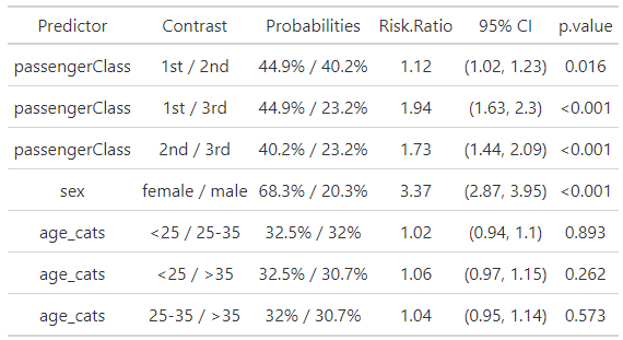
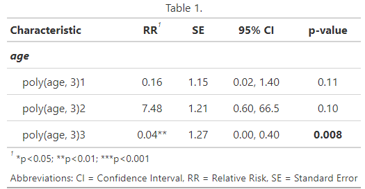
Multivariable Code
# Polynomial Table ################### tab_poly <- tbl_regression( m_poly, exponentiate = TRUE, add_pairwise_contrasts = TRUE, pairwise_reverse = FALSE ) |> add_significance_stars( hide_p = FALSE, hide_se = FALSE, hide_ci = FALSE ) |> modify_header(lable = "**Predictor**") |> modify_caption("Table 1.") |> modify_footnote(abbreviation = TRUE) |> bold_labels() |> italicize_labels() |> bold_p() tab_poly # Multivariable Table ################### logbin_table <- function(data, formula, smooth = FALSE) { m <- logbin(formula, data = data) # extract predictor names predictors <- all.vars(formula)[-1] all_contrasts <- list() all_prob_pairs <- list() all_predictors <- list() all_contrast_labels <- list() for (pred in predictors) { emm <- emmeans( m, as.formula(paste("pairwise ~", pred)), type = "response", weights = "prop", infer = TRUE ) contrasts <- summary(emm$contrasts, infer = TRUE) probs <- summary(emm$emmeans, type = "response") probs_formatted <- paste0(round(probs$prob * 100, 1), "%") # contrast labels and prob pairs levels <- as.character(probs[[pred]]) contrast_labels <- c() prob_pairs <- c() for (i in 1:(length(levels) - 1)) { for(j in (i+1):length(levels)) { contrast_labels <- c(contrast_labels, paste(levels[i], "/", levels[j])) prob_pairs <- c(prob_pairs, paste(probs_formatted[i], "/", probs_formatted[j])) } } all_contrasts[[pred]] <- contrasts all_prob_pairs[[pred]] <- prob_pairs all_predictors[[pred]] <- rep(pred, length(prob_pairs)) all_contrast_labels[[pred]] <- contrast_labels } table <- data.frame( Predictor = unlist(all_predictors), Contrast = unlist(all_contrast_labels), Probabilities = unlist(all_prob_pairs), `Risk Ratio` = round(unlist(lapply( all_contrasts, function(x) x$ratio )), 2), ci_95 = paste0("(", round(unlist(lapply( all_contrasts, function(x) x$asymp.LCL )), 2), ", ", round(unlist(lapply( all_contrasts, function(x) x$asymp.UCL )), 2), ")"), `p.value` = ifelse(unlist(lapply( all_contrasts, function(x) x$p.value )) < 0.001, "<0.001", round(unlist(lapply( all_contrasts, function(x) x$p.value )), 3)) ) |> as_gtsummary() |> modify_header(ci_95 ~ "95% CI") return(table) } d_bal <- d |> mutate( age_cats = case_when( age < 25 ~ "<25", between(age, 25, 35) ~ "25-35", age > 35 ~ ">35"), age_cats = factor(age_cats, levels = c("<25", "25-35", ">35"))) tab_spl_multi <- logbin_table( data = d_bal, formula = survived ~ passengerClass + sex + age_cats ) tab_spl_multi- The
logbin_tablefunction doesn’t supportlogbin.smooth, so instead of fitting simple model, I decided to fit a multivariable model to fill out the table a little bit to see what it looks like. - The code for
logbin_tableis ridiculously long with nested for-loops (not coded by me). {marginaleffects} outputs tibbles/dataframes or at least I think they can be easily extracted. So, if I were to rewrite this function so I could use logbin.smooth, then I think that might be an easier route for bothlogbinandlogbin.smooth. - The major benefit of something like
logbin_tableis that it shows you the contrasts and probabilities that are used for the risk ratio calculation.
Marginal Means
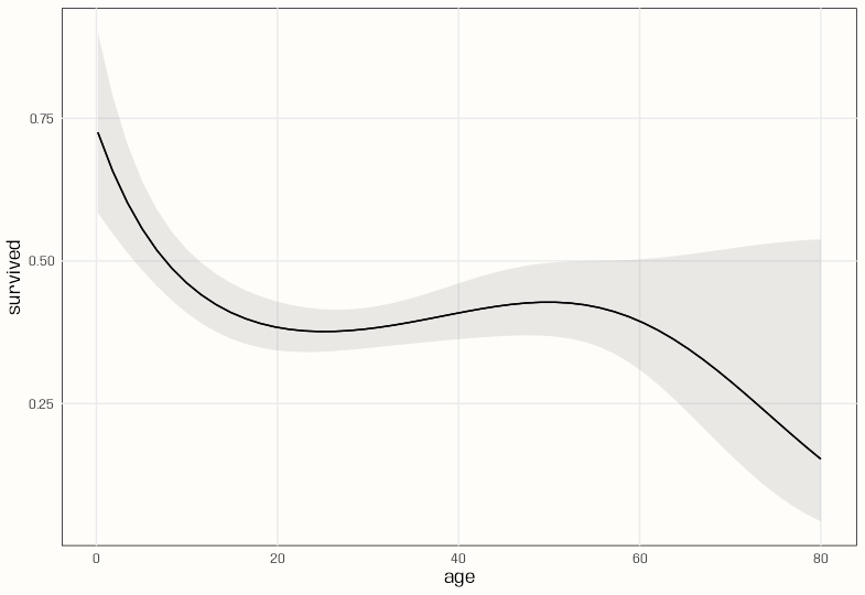
Polynomial 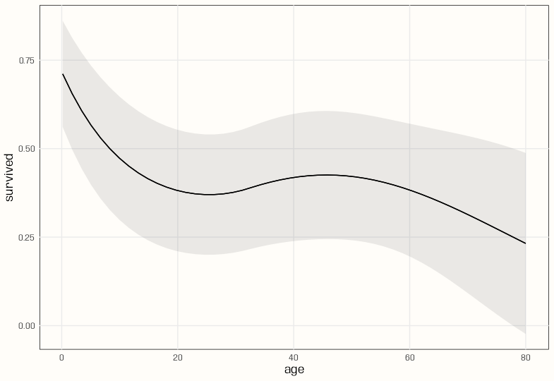
B-Spline plot_predictions(m_poly, condition = "age") plot_predictions(m_spl_bin, condition = "age")- There seems to be a lot more curvature with the polynomial, and the CI bands are narrower. Both have similar shapes.
Slopes
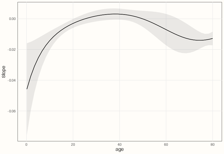
poly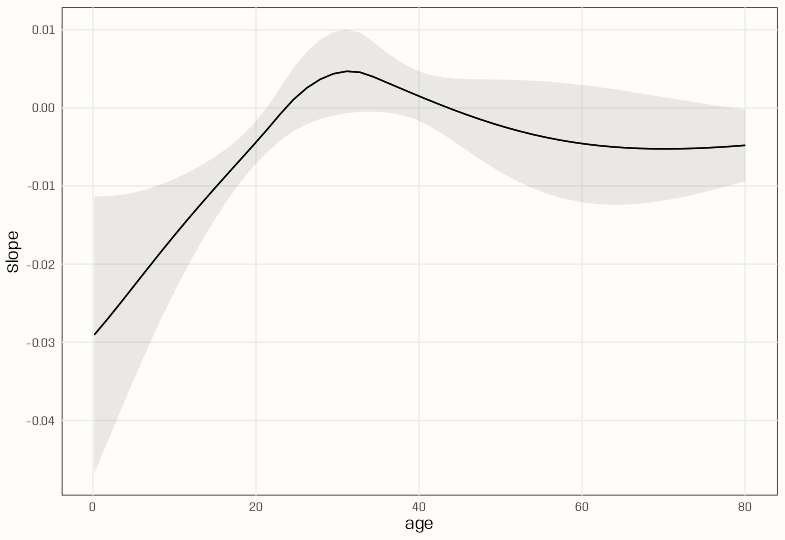
nsplot_slopes(m_poly, variables = "age", condition = "age") m_spl <- glm(survived ~ splines::ns(age, df = 3), data = d, family = binomial(link = "log")) plot_slopes(m_spl, variables = "age", condition = "age")- Unfortuneately, slopes at the unit level can’t be calculated for a
logbin.smoothobject. I think it’s a bug. - Switching to a
glmand natural spline does work. - The polynomial has a smoother slope across age values and peaks a little later than the natural spline.
- The slope for the polynomial model stays positive over a larger range than the natural spline model — about age 25 to 50.
Example 2: Interactions
pacman::p_load( dplyr, ggplot2, emmeans, marginaleffects, sjPlot ) theme_set(theme_notebook()) notebook_colors <- unname(swatches::read_ase(here::here("palettes/Forest Floor.ase"))) d <- d |> mutate(age_cats = case_when( age < 10 ~ "<10", between(age, 10, 30) ~ "10-30", age > 30 ~ ">30"), age_cats = factor(age_cats, levels = c("<10", "10-30", ">30"))) m_bin_int <- glm(survived ~ passengerClass * age_cats, data = d, family = binomial(link = "log"), start = c(log(0.5), 0, 0, 0, 0, 0, 0, 0, 0)) m_spl_int <- glm(survived ~ passengerClass * splines::ns(age, df = 3), data = d, family = binomial(link = "log"), control = glm.control(maxit = 200), start = c(log(0.5), rep(0, 11))) range(fitted(m_spl_int)) #> [1] 0.04274709 1.00000000 range(fitted(m_bin_int)) #> [1] 0.1897812 0.9999998 sum(fitted(m_spl_int) == 1) #> [1] 0 sum(round(fitted(m_spl_int), 3) == 1.000) #> [1] 1 which(round(fitted(m_spl_int), 3) == 1) #> Hamalainen, Master. Viljo #> 385- The model with the spline interaction didn’t converge at first. So, I increased the iterations (default maxit is 25).
- The converged models had two warnings:
- “algorithm stopped at boundary value” which indicates that one or more parameter estimates hit a boundary during optimization.
- This likely means some estimates became very large (approaching infinity) or hit computational limits.
summary(m_bin_inter)andsummary(m_spl_inter)showed out of both models the largest magnitude of an effect is only 1.99. No extreme parameter estimates (e.g. -10, 20) likely indicates no separation has occurred. A stable solution was found and the effect estimates should be reliable.
- This likely means some estimates became very large (approaching infinity) or hit computational limits.
- “fitted probabilities numerically 0 or 1 occurred”
- Only one observation in the spline interaction model has a combination of passenger class and age that the model predicts with near-certainty for survival (or non-survival) (which triggered the warning)
- “algorithm stopped at boundary value” which indicates that one or more parameter estimates hit a boundary during optimization.
- Both models seems fine regarding the concerns raised by the warnings.
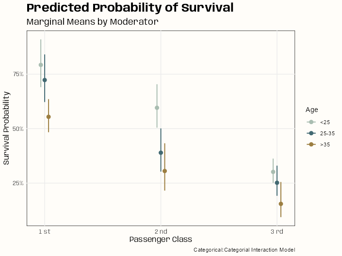
# cat:cat interaction emmeans( m_bin_int, pairwise ~ passengerClass | age_cats, type = "response", weights = "prop", infer = TRUE ) #> $emmeans #> age_cats = <10: #> passengerClass prob SE df asymp.LCL asymp.UCL null z.ratio p.value #> 1st 0.75000 0.217000 Inf 0.42593 1.32063 1 -0.997 0.3190 #> 2nd 1.00000 0.000117 Inf 0.99977 1.00023 1 -0.001 0.9990 #> 3rd 0.44643 0.066400 Inf 0.33349 0.59761 1 -5.420 <.0001 #> #> age_cats = 10-30: #> passengerClass prob SE df asymp.LCL asymp.UCL null z.ratio p.value #> 1st 0.72941 0.048200 Inf 0.64083 0.83024 1 -4.776 <.0001 #> 2nd 0.41791 0.042600 Inf 0.34222 0.51035 1 -8.558 <.0001 #> 3rd 0.25974 0.025000 Inf 0.21511 0.31363 1 -14.014 <.0001 #> #> age_cats = >30: #> passengerClass prob SE df asymp.LCL asymp.UCL null z.ratio p.value #> 1st 0.59487 0.035200 Inf 0.52981 0.66792 1 -8.789 <.0001 #> 2nd 0.35238 0.046600 Inf 0.27189 0.45670 1 -7.884 <.0001 #> 3rd 0.18978 0.033500 Inf 0.13427 0.26823 1 -9.414 <.0001 #> #> Confidence level used: 0.95 #> Intervals are back-transformed from the log scale #> Tests are performed on the log scale #> #> $contrasts #> age_cats = <10: #> contrast ratio SE df asymp.LCL asymp.UCL null z.ratio p.value #> 1st / 2nd 0.75 0.217 Inf 0.381 1.48 1 -0.997 0.5790 #> 1st / 3rd 1.68 0.546 Inf 0.785 3.60 1 1.597 0.2467 #> 2nd / 3rd 2.24 0.333 Inf 1.580 3.17 1 5.420 <.0001 #> #> age_cats = 10-30: #> contrast ratio SE df asymp.LCL asymp.UCL null z.ratio p.value #> 1st / 2nd 1.75 0.212 Inf 1.313 2.32 1 4.585 <.0001 #> 1st / 3rd 2.81 0.328 Inf 2.136 3.69 1 8.848 <.0001 #> 2nd / 3rd 1.61 0.226 Inf 1.158 2.23 1 3.393 0.0020 #> #> age_cats = >30: #> contrast ratio SE df asymp.LCL asymp.UCL null z.ratio p.value #> 1st / 2nd 1.69 0.245 Inf 1.202 2.37 1 3.614 0.0009 #> 1st / 3rd 3.13 0.584 Inf 2.026 4.85 1 6.137 <.0001 #> 2nd / 3rd 1.86 0.410 Inf 1.107 3.11 1 2.805 0.0139 # cont:cat interaction emmeans( m_spl_int, pairwise ~ age | passengerClass, at = list(age = c(quantile(d$age, probs = c(0.05, 0.50, 0.95)))), type = "response", weights = "prop", infer = TRUE ) #> $emmeans #> passengerClass = 1st: #> age prob SE df asymp.LCL asymp.UCL null z.ratio p.value #> 5 0.820 0.1500 Inf 0.5729 1.173 1 -1.087 0.2772 #> 28 0.726 0.0402 Inf 0.6510 0.809 1 -5.786 <.0001 #> 57 0.507 0.0508 Inf 0.4166 0.617 1 -6.774 <.0001 #> #> passengerClass = 2nd: #> age prob SE df asymp.LCL asymp.UCL null z.ratio p.value #> 5 0.817 0.0350 Inf 0.7513 0.889 1 -4.715 <.0001 #> 28 0.415 0.0366 Inf 0.3490 0.493 1 -9.981 <.0001 #> 57 0.220 0.0788 Inf 0.1088 0.444 1 -4.226 <.0001 #> #> passengerClass = 3rd: #> age prob SE df asymp.LCL asymp.UCL null z.ratio p.value #> 5 0.420 0.0548 Inf 0.3254 0.542 1 -6.653 <.0001 #> 28 0.235 0.0244 Inf 0.1917 0.288 1 -13.936 <.0001 #> 57 0.100 0.0675 Inf 0.0267 0.375 1 -3.412 0.0006 #> #> Confidence level used: 0.95 #> Intervals are back-transformed from the log scale #> Tests are performed on the log scale #> #> $contrasts #> passengerClass = 1st: #> contrast ratio SE df asymp.LCL asymp.UCL null z.ratio p.value #> age5 / age28 1.13 0.229 Inf 0.702 1.82 1 0.601 0.8193 #> age5 / age57 1.62 0.336 Inf 0.994 2.63 1 2.313 0.0540 #> age28 / age57 1.43 0.169 Inf 1.085 1.89 1 3.036 0.0068 #> #> passengerClass = 2nd: #> contrast ratio SE df asymp.LCL asymp.UCL null z.ratio p.value #> age5 / age28 1.97 0.164 Inf 1.621 2.39 1 8.161 <.0001 #> age5 / age57 3.72 1.320 Inf 1.619 8.54 1 3.702 0.0006 #> age28 / age57 1.89 0.723 Inf 0.769 4.63 1 1.658 0.2214 #> #> passengerClass = 3rd: #> contrast ratio SE df asymp.LCL asymp.UCL null z.ratio p.value #> age5 / age28 1.79 0.307 Inf 1.197 2.67 1 3.390 0.0020 #> age5 / age57 4.20 2.880 Inf 0.842 20.95 1 2.092 0.0914 #> age28 / age57 2.35 1.660 Inf 0.447 12.34 1 1.206 0.4497- Marginal means in the first section and risk ratios in the second section.
- For the m_bin_int, we nterestingly see a 1.0 probability average for a second class passenger less than 10 yrs old. This model didn’t have any 1.0 predicitons, but it turns it out it did have 22 99% predictions. Guessing there’s some rounding. (m_spl_int only had 3.)
- The marginal means of both models are not close to agreement, but the order of probabilities (i.e. largest to smallest) agrees.
- For m_bin_int, a 28 yr old in second class has 41.5% chance of survival on average.
- Reminder: emmeans p-values for marginal means don’t make sense in this case, since the null is 1.
- For m_spl_int, a 28 yr old in 3rd Class was 2.35 times (or 135%) more likely to survive than a 57 yr old in 3rd Class
Marginal Means and Risk Ratios
# marginal means by moderator ## cat:cat interaction mm_bin_int <- avg_predictions(m_bin_int, by = c("age_cats", "passengerClass")) ## cont:cat interaction mm_spl_int <- avg_predictions(m_spl_int, variables = list(age = c(5, 28, 57)), by = c("age", "passengerClass")) |> arrange(passengerClass) # risk ratios by moderator ## cat:cat interaction rr_bin_int <- avg_comparisons(m_bin_int, variables = list(passengerClass = "revpairwise"), by = "age_cats", comparison = "ratioavg") |> arrange(age_cats) ## cont:cat interaction rr_spl_int <- avg_predictions( m_spl_int, variables = list(age = c(5, 28, 57)), by = c("age", "passengerClass"), hypothesis = ratio ~ revpairwise | passengerClass )- The marginal means and risk ratios match the emmeans output, so I didn’t repeat it here
Risk Differences
# cat:cat interaction rd_bin_int <- avg_predictions(m_bin_int, variables = "passengerClass", hypothesis = difference ~ revpairwise) #> Hypothesis Estimate Std. Error z Pr(>|z|) S 2.5 % 97.5 % #> (1st) - (2nd) 0.239 0.0440 5.43 <0.001 24.1 0.152 0.325 #> (1st) - (3rd) 0.430 0.0384 11.19 <0.001 94.1 0.354 0.505 #> (2nd) - (3rd) 0.191 0.0350 5.47 <0.001 24.4 0.123 0.260 #> #> Type: response # cont:cat interaction rd_spl_int <- comparisons(m_spl_int, variables = "age", newdata = datagrid(age = c(5, 28, 57)), hypothesis = difference ~ revpairwise) #> Hypothesis Estimate Std. Error z Pr(>|z|) S 2.5 % 97.5 % #> (b1) - (b2) -0.01091 0.01061 -1.028 0.304 1.7 -0.0317 0.00989 #> (b1) - (b3) -0.00972 0.00717 -1.354 0.176 2.5 -0.0238 0.00434 #> (b2) - (b3) 0.00119 0.00631 0.189 0.850 0.2 -0.0112 0.01356 #> #> Type: response # By moderator # cat:cat interaction rd_mod_bin_int <- avg_comparisons(m_bin_int, variables = list(passengerClass = "revpairwise"), by = "age_cats") rd_mod_bin_int #> Contrast age_cats Estimate Std. Error z Pr(>|z|) S 2.5 % 97.5 % #> 1st - 2nd <10 -0.250 0.2165 -1.15 0.24821 2.0 -0.6743 0.174 #> 1st - 3rd <10 0.304 0.2265 1.34 0.18010 2.5 -0.1403 0.747 #> 2nd - 3rd <10 0.554 0.0664 8.33 < 0.001 53.5 0.4234 0.684 #> 1st - 2nd 10-30 0.312 0.0643 4.84 < 0.001 19.6 0.1854 0.438 #> 1st - 3rd 10-30 0.470 0.0543 8.65 < 0.001 57.5 0.3633 0.576 #> 2nd - 3rd 10-30 0.158 0.0494 3.20 0.00136 9.5 0.0614 0.255 #> 1st - 2nd >30 0.242 0.0584 4.15 < 0.001 14.9 0.1280 0.357 #> 1st - 3rd >30 0.405 0.0486 8.34 < 0.001 53.6 0.3099 0.500 #> 2nd - 3rd >30 0.163 0.0574 2.83 0.00462 7.8 0.0501 0.275 #> #> Term: passengerClass #> Type: response # cont:cat interaction rd_mod_spl_int <- avg_comparisons(m_spl_int, variables = list(passengerClass = "revpairwise"), newdata = datagrid(age = c(5, 28, 57)), by = "age") rd_mod_spl_int #> Contrast age Estimate Std. Error z Pr(>|z|) S 2.5 % 97.5 % #> 1st - 2nd 5 0.00267 0.1539 0.0173 0.98617 0.0 -0.2991 0.304 #> 1st - 3rd 5 0.39965 0.1596 2.5041 0.01228 6.3 0.0868 0.712 #> 2nd - 3rd 5 0.39698 0.0650 6.1082 < 0.001 29.9 0.2696 0.524 #> 1st - 2nd 28 0.31084 0.0544 5.7186 < 0.001 26.5 0.2043 0.417 #> 1st - 3rd 28 0.49072 0.0470 10.4305 < 0.001 82.2 0.3985 0.583 #> 2nd - 3rd 28 0.17988 0.0440 4.0908 < 0.001 14.5 0.0937 0.266 #> 1st - 2nd 57 0.28728 0.0938 3.0639 0.00218 8.8 0.1035 0.471 #> 1st - 3rd 57 0.40697 0.0845 4.8163 < 0.001 19.4 0.2414 0.573 #> 2nd - 3rd 57 0.11969 0.1037 1.1537 0.24861 2.0 -0.0836 0.323 #> #> Term: passengerClass #> Type: response- On average, moving from 2nd to 1st class is associated with a decrease of 23.9% in probability of survival. This difference is significant.
- On average, moving from 1st to 2nd class is associated with a decrease of 25% in probability of survival when the passenger is younger that 10 yrs old. This difference is not significant.
Marginal Effects
# marginal effects # cont-cat interaction me_spl_int <- slopes(m_spl_int, variables = "age", newdata = datagrid(age = c(5, 28, 57))) #> age Estimate Std. Error z Pr(>|z|) S 2.5 % 97.5 % #> 5 -0.01447 0.00817 -1.771 0.0766 3.7 -0.0305 0.00154 #> 28 -0.00328 0.00398 -0.824 0.4100 1.3 -0.0111 0.00452 #> 57 -0.00451 0.00283 -1.593 0.1112 3.2 -0.0101 0.00104 #> #> Term: age #> Type: response # by moderator # cont:cat interaction me_mod_spl_int <- slopes( m_spl_int, variables = "age", newdata = datagrid(age = c(5, 28, 57), passengerClass = unique) ) #> age passengerClass Estimate Std. Error z Pr(>|z|) S 2.5 % 97.5 % #> 5 1st -0.00138 0.01419 -0.0971 0.9227 0.1 -0.0292 0.02643 #> 5 2nd -0.03739 0.00605 -6.1747 <0.001 30.5 -0.0493 -0.02552 #> 5 3rd -0.01447 0.00817 -1.7709 0.0766 3.7 -0.0305 0.00154 #> 28 1st -0.00757 0.00555 -1.3626 0.1730 2.5 -0.0185 0.00332 #> 28 2nd -0.00343 0.00610 -0.5619 0.5742 0.8 -0.0154 0.00852 #> 28 3rd -0.00328 0.00398 -0.8238 0.4100 1.3 -0.0111 0.00452 #> 57 1st -0.00677 0.00487 -1.3913 0.1641 2.6 -0.0163 0.00277 #> 57 2nd -0.00820 0.00471 -1.7401 0.0818 3.6 -0.0174 0.00104 #> 57 3rd -0.00451 0.00283 -1.5928 0.1112 3.2 -0.0101 0.00104 #> #> Term: age #> Type: response #> Comparison: dY/dX # ratio of marginal effects # cont:cat interacion slopes( m_spl_int, variables = "age", newdata = datagrid(age = c(5, 28, 57), passengerClass = unique), hypothesis = ratio ~ revpairwise | passengerClass ) #> passengerClass Hypothesis Estimate Std. Error z Pr(>|z|) S 2.5 % 97.5 % #> 1st (b1) / (b4) 0.182 1.94 0.0936 0.9254 0.1 -3.627 3.99 #> 1st (b1) / (b7) 0.203 2.05 0.0990 0.9211 0.1 -3.823 4.23 #> 1st (b4) / (b7) 1.118 1.51 0.7410 0.4587 1.1 -1.839 4.08 #> 2nd (b2) / (b5) 10.912 21.00 0.5197 0.6033 0.7 -30.245 52.07 #> 2nd (b2) / (b8) 4.561 2.27 2.0075 0.0447 4.5 0.108 9.01 #> 2nd (b5) / (b8) 0.418 0.95 0.4400 0.6599 0.6 -1.444 2.28 #> 3rd (b3) / (b6) 4.417 7.11 0.6211 0.5345 0.9 -9.522 18.36 #> 3rd (b3) / (b9) 3.212 2.09 1.5344 0.1249 3.0 -0.891 7.31 #> 3rd (b6) / (b9) 0.727 1.28 0.5679 0.5701 0.8 -1.783 3.24 #> #> Type: response- The average effect of increasing the age by 1 unit for 5yr olds is a decrease of 0.01447 on the predicted probability of survival.
- The average effect of increasing the age by 1 unit for 5yr olds in second class is a decrease of 0.03739 on the predicted probablity of survival.
- The “b” labels for the age values are annoying, but I couldn’t figure out how to get rid of them and still get the desired output. See “by moderator” age values in the section above it for a mapping of the b labels the age label
- e.g. age 5 and 1st class is b1, age 28 in 1st class is b4, etc.
- A 28 year old person in 1st class is 1.118 times (11.8%) more likely to survive than a 57 year old person in 1st class.
- Other (using refit models)
Average slope of age for each passenger class:
slopes(m_spl_int_cent, variables = "age_cent", by = "passengerClass")
#>  passengerClass Estimate Std. Error    z Pr(>|z|)    S    2.5 %   97.5 %
#>             1st -0.00689    0.00186 -3.7   <0.001 12.2 -0.01053 -0.00324
#>             2nd -0.00988    0.00210 -4.7   <0.001 18.5 -0.01400 -0.00576
#>             3rd -0.00617    0.00176 -3.5   <0.001 11.1 -0.00963 -0.00271
#>
#> Term: age_cent
#> Type:  response
#> Comparison: dY/dX
Difference in age slope when moving from 2nd to 1st passenger class and 3rd to 1st passenger class
slopes(m_spl_int_cent, variables = "passengerClass", by = "age_cent") #> Contrast age_cent Estimate Std. Error z Pr(>|z|) S 2.5 % 97.5 % #> 2nd - 1st -29.7 0.198 0.215 0.920 0.35759 1.5 -0.224 0.6205 #> 3rd - 1st -29.7 -0.328 0.235 -1.394 0.16322 2.6 -0.789 0.1331 #> 2nd - 1st -29.5 0.190 0.213 0.894 0.37154 1.4 -0.227 0.6080 #> 3rd - 1st -29.5 -0.331 0.232 -1.423 0.15469 2.7 -0.787 0.1248 #> 2nd - 1st -29.5 0.186 0.212 0.880 0.37872 1.4 -0.229 0.6017 #> --- 186 rows omitted. See ?print.marginaleffects --- #> 3rd - 1st 44.1 -0.359 0.139 -2.589 0.00963 6.7 -0.631 -0.0873 #> 2nd - 1st 46.1 -0.293 0.162 -1.809 0.07050 3.8 -0.611 0.0245 #> 3rd - 1st 46.1 -0.353 0.144 -2.441 0.01463 6.1 -0.636 -0.0695 #> 2nd - 1st 50.1 -0.289 0.172 -1.681 0.09269 3.4 -0.625 0.0478 #> 3rd - 1st 50.1 -0.339 0.155 -2.186 0.02883 5.1 -0.643 -0.0350 #> Term: passengerClass #> Type: response- This is the data for
plot_slopes(m_spl_int_cent, variables = "passengerClass", condition = "age_cent")
- This is the data for
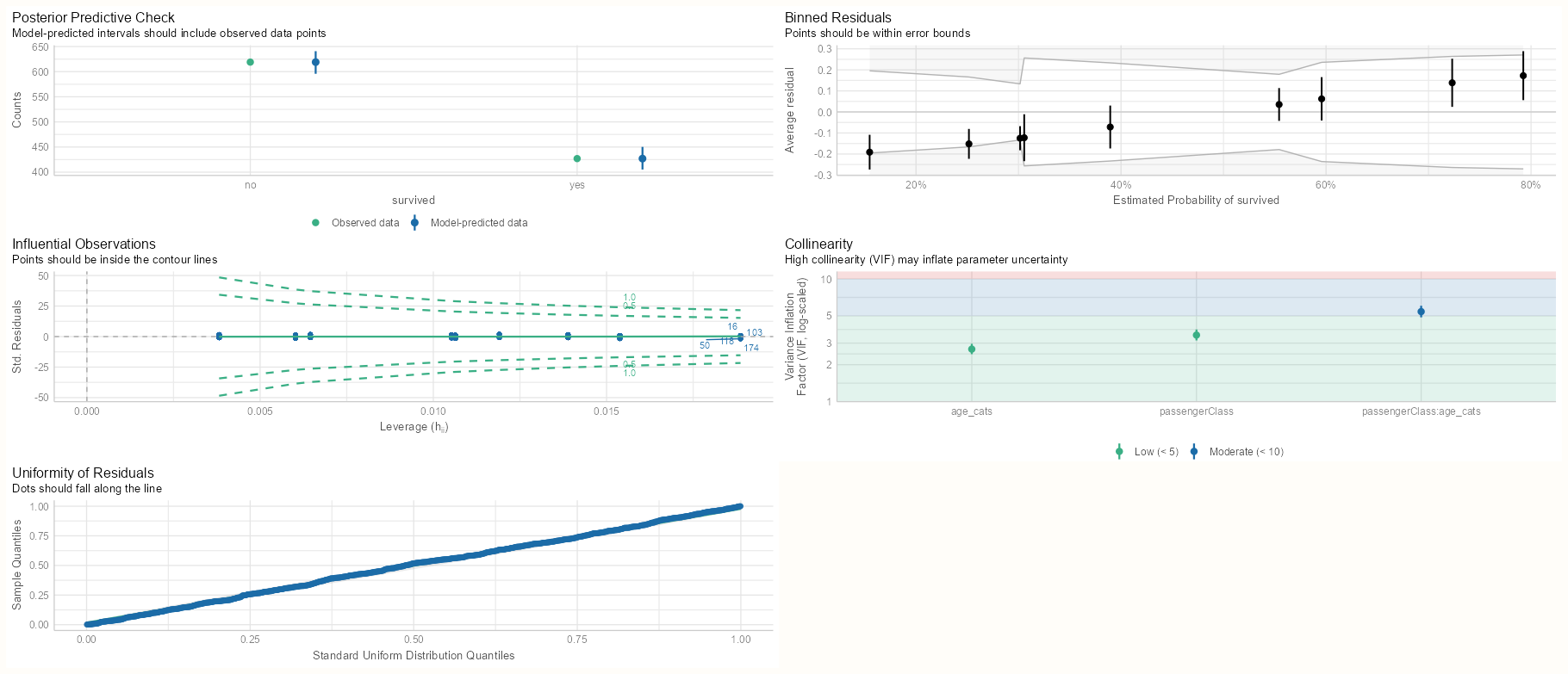
Diagnostics
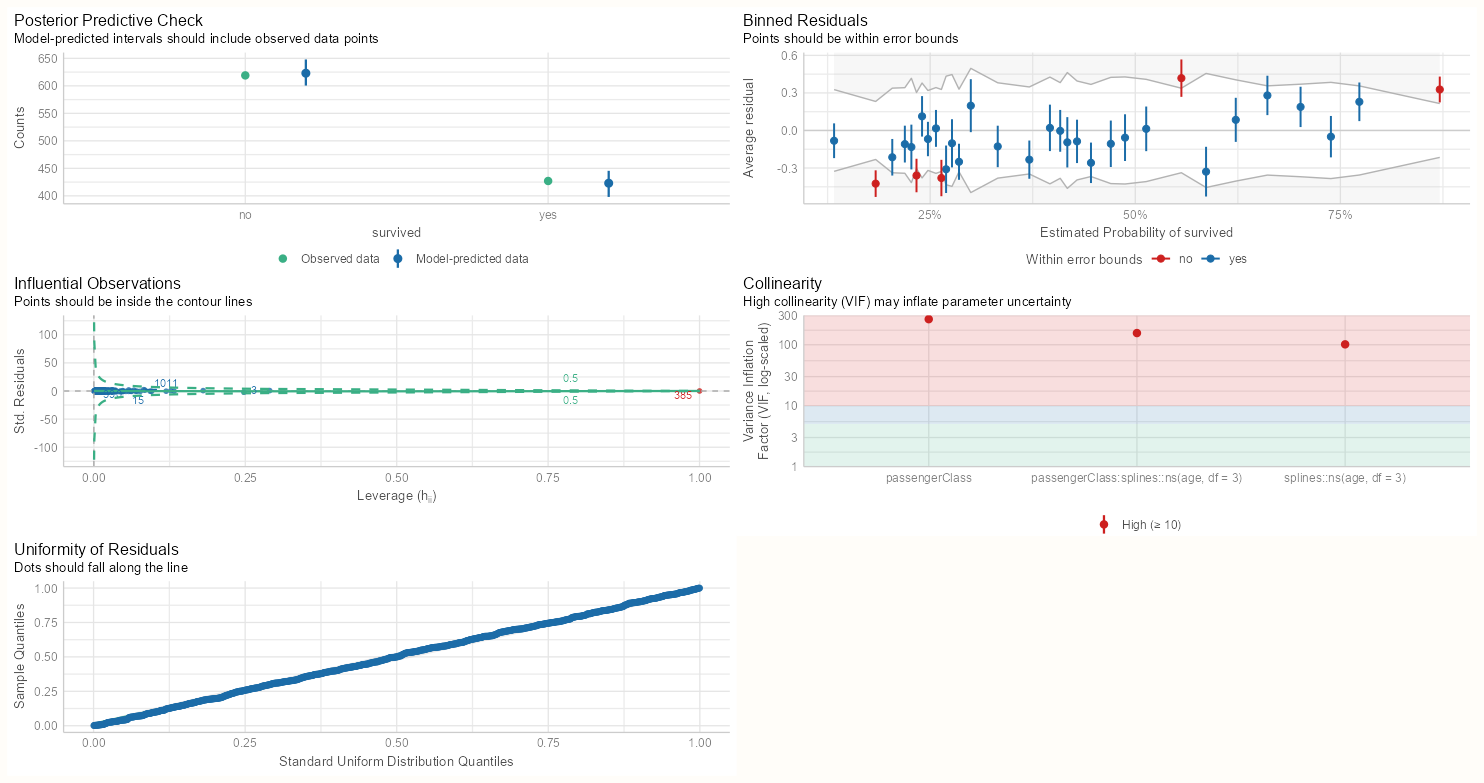
Binned Age Splined Age performance::check_model(m_bin_int) performance::check_model(m_spl_int)- Both models have five extreme residuals
- Both models have very high VIF scores for their interactions and main effects. We’re reminded in the subtitle that high VIF scores can inflate our standard errors.
- This is expected in the continuous:categorical interaction, so we’ll need to center the numeric variable to hopefully get rid of the collinearity between the interaction and the main effects.
- For categorical:categorical interaction, the high VIF is likely caused by an extreme imbalance in the 2x2 cell counts.
- That one observation with a fitted value of one (see Data and Model tab) is identified as an influential value
Re-bin and Center
summarytools::ctable(d$passengerClass, d$age_cats) #> ---------------- ---------- ------------ ------------- ------------- --------------- #> age_cats <10 10-30 >30 Total #> passengerClass #> 1st 4 ( 1.4%) 85 (29.9%) 195 (68.7%) 284 (100.0%) #> 2nd 22 ( 8.4%) 134 (51.3%) 105 (40.2%) 261 (100.0%) #> 3rd 56 (11.2%) 308 (61.5%) 137 (27.3%) 501 (100.0%) #> Total 82 ( 7.8%) 527 (50.4%) 437 (41.8%) 1046 (100.0%) #> ---------------- ---------- ------------ ------------- ------------- --------------- # rebin d_bal <- d |> mutate(age_cats = case_when( age < 25 ~ "<25", between(age, 25, 35) ~ "25-35", age > 35 ~ ">35"), age_cats = factor(age_cats, levels = c("<25", "25-35", ">35"))) summarytools::ctable(d_bal$passengerClass, d_bal$age_cats) #> ---------------- ---------- ------------- ------------- ------------- --------------- #> age_cats <25 25-35 >35 Total #> passengerClass #> 1st 53 (18.7%) 65 (22.9%) 166 (58.5%) 284 (100.0%) #> 2nd 94 (36.0%) 95 (36.4%) 72 (27.6%) 261 (100.0%) #> 3rd 262 (52.3%) 155 (30.9%) 84 (16.8%) 501 (100.0%) #> Total 409 (39.1%) 315 (30.1%) 322 (30.8%) 1046 (100.0%) #> ---------------- ---------- ------------- ------------- ------------- --------------- # center d_cent <- d |> mutate(age_cent = as.numeric(scale(age, scale = FALSE)))- The cells in the <10 column have relatively low counts. We could collapse the <10 category with the 10-30 category, but most of the 10-30 cells already have at least 50% of the counts. Therefore collapsing may not be optimal and could exacerbate the issue.
- Instead, the outer bins are given observations from the inner bin.
- Age was centered
- Tried removing the influential observation, but there wasn’t much of difference in terms of performance.
Refit and Check
Binned Age, Balanced 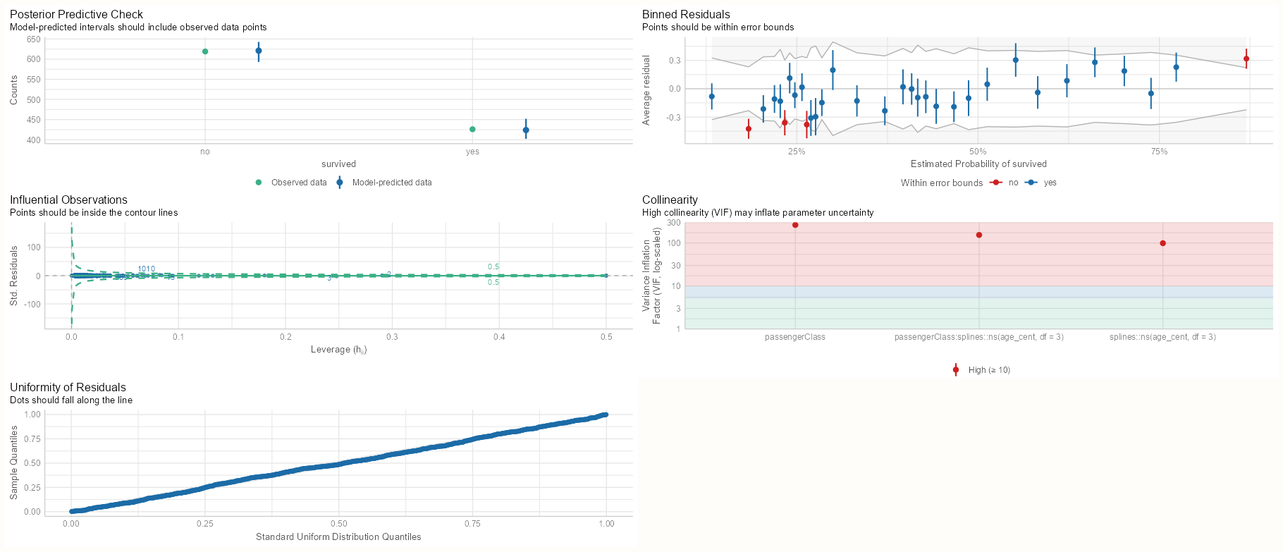
Splined Age, Centered m_bin_int_bal <- glm(survived ~ passengerClass * age_cats, data = d_bal2, family = binomial(link = "log")) m_spl_int_cent <- glm(survived ~ passengerClass * splines::ns(age_cent, df = 3), data = d_cent, family = binomial(link = "log"), control = glm.control(maxit = 200), start = c(log(0.5), rep(0, 11))) summary(m_bin_int_bal) #> Estimate Std. Error z value Pr(>|z|) #> (Intercept) -0.23262 0.07030 -3.309 0.000936 *** #> passengerClass2nd -0.28532 0.11027 -2.587 0.009671 ** #> passengerClass3rd -0.96627 0.11740 -8.231 < 2e-16 *** #> age_cats25-35 -0.09162 0.10408 -0.880 0.378739 #> age_cats>35 -0.35758 0.09893 -3.614 0.000301 *** #> passengerClass2nd:age_cats25-35 -0.33340 0.18588 -1.794 0.072881 . #> passengerClass3rd:age_cats25-35 -0.08935 0.19714 -0.453 0.650385 #> passengerClass2nd:age_cats>35 -0.31010 0.22039 -1.407 0.159407 #> passengerClass3rd:age_cats>35 -0.30939 0.28922 -1.070 0.284726 #> --- #> #> Null deviance: 1414.6 on 1045 degrees of freedom #> Residual deviance: 1269.5 on 1037 degrees of freedom #> AIC: 1287.5 summary(m_spl_int_cent) #> Estimate Std. Error z value Pr(>|z|) #> (Intercept) -0.1916 0.2609 -0.734 0.4627 #> passengerClass2nd 0.2152 0.2609 0.825 0.4096 #> passengerClass3rd -0.5066 0.3231 -1.568 0.1169 #> splines::ns(age_cent, df = 3)1 -0.3161 0.2179 -1.451 0.1469 #> splines::ns(age_cent, df = 3)2 -0.6128 0.5891 -1.040 0.2982 #> splines::ns(age_cent, df = 3)3 -0.7901 0.3923 -2.014 0.0440 * #> passengerClass2nd:splines::ns(age_cent, df = 3)1 -0.2819 0.4746 -0.594 0.5525 #> passengerClass3rd:splines::ns(age_cent, df = 3)1 -0.3467 0.5509 -0.629 0.5291 #> passengerClass2nd:splines::ns(age_cent, df = 3)2 -1.9940 0.8796 -2.267 0.0234 * #> passengerClass3rd:splines::ns(age_cent, df = 3)2 -1.9206 1.3759 -1.396 0.1627 #> passengerClass2nd:splines::ns(age_cent, df = 3)3 -1.3104 1.2480 -1.050 0.2937 #> passengerClass3rd:splines::ns(age_cent, df = 3)3 -1.6627 2.1551 -0.772 0.4404 #> --- #> Null deviance: 1414.6 on 1045 degrees of freedom #> Residual deviance: 1239.5 on 1034 degrees of freedom #> AIC: 1263.5- (Not shown) For the centered age model, the marginal means, slopes, and their contrasts are the same. The only thing you need to do for any table or visualization is back-transform the centered values back to the orginal ages (add mean to age value).
- For rebinned model, everything looks great. Rebalancing cured everything
- For the centered model, unfortunately, there was little effect. VIF scores are still high and four extreme residuals remain.
- Tried using
polythinking the orthogonal contrasts might help, but the result was pretty much the same.
- Tried using
- In neither model’s summary do we see extreme coefficients or standard errors, so the models should be fairly reliable for interpretation.
- In the binned model summary, the significant effects have switched from the interaction variables to the main effects.
- In the spline model summary, the coefficients are very close to the previous model. The standard errors are pretty high, so we only see a couple estimates that are barely significant.
- Residual Deviance favors the spline model.
Score
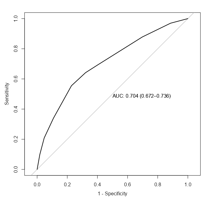
Binned Age, Balanced 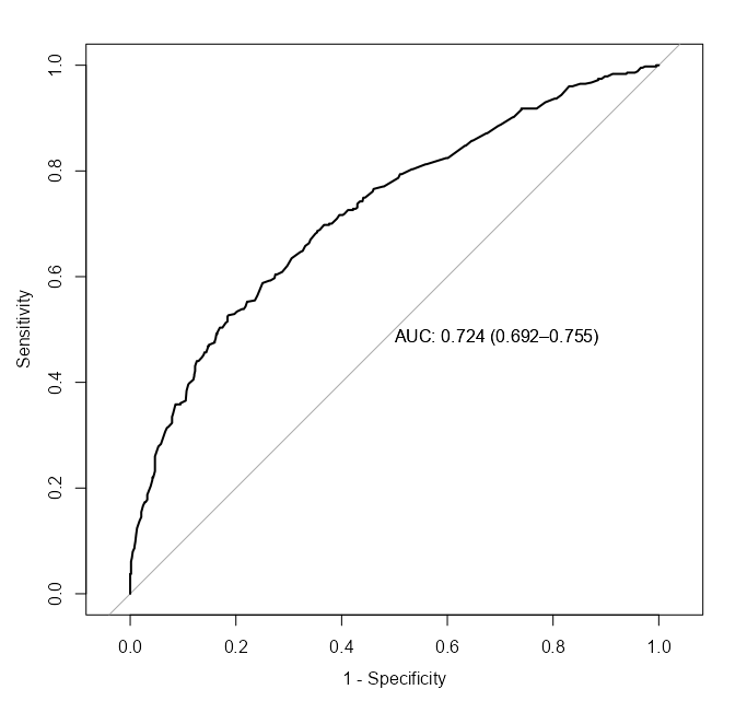
Splined Age, Centered pROC::roc( survived ~ fitted.values(m_bin_int_bal), data = d, plot = TRUE, legacy.axes = TRUE, print.auc = TRUE, ci = TRUE ) pROC::roc( survived ~ fitted.values(m_spl_int_cent), data = d, plot = TRUE, legacy.axes = TRUE, print.auc = TRUE, ci = TRUE ) performance::compare_performance(m_bin_int_bal, m_spl_int_cent) #> Name | Model | AIC (weights) | AICc (weights) | BIC (weights) | Nagelkerke's R2 | RMSE | Sigma | Log_loss #> ---------------------------------------------------------------------------------------------------------------------- #> m_bin_int_bal | glm | 1287.5 (<.001) | 1287.7 (<.001) | 1332.1 (0.010) | 0.175 | 0.457 | 1.000 | 0.607 #> m_spl_int_cent | glm | 1263.5 (>.999) | 1263.8 (>.999) | 1322.9 (0.990) | 0.208 | 0.451 | 1.000 | 0.592 #> #> Name | Score_log | Score_spherical | PCP #> ---------------------------------------------------- #> m_bin_int_bal | -247.482 | 0.004 | 0.582 #> m_spl_int_cent | -Inf | 9.752e-04 | 0.592- The spline model has a better point estimate of the AUC, but is within the CI of the binned model.
- The spline model has a slightly better AICc and R2.
Marginal Means
Binned Age, Balanced 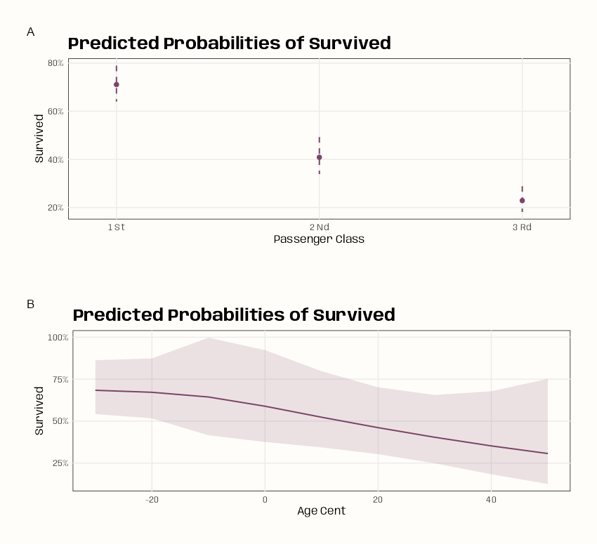
Splined Age, Centered Code
ggeffects::ggeffect(m_bin_int_bal) |> plot( use_theme = FALSE, colors = notebook_colors[[5]], case = "title" ) |> sjPlot::plot_grid() ggeffects::ggeffect(m_spl_int_cent) |> plot( use_theme = FALSE, colors = notebook_colors[[9]], case = "title", ) |> sjPlot::plot_grid(tags = FALSE)- In the Splined Age model, the X-axis labels show the centered age values. There doesn’t seem to be an argument in the
plotfunction that allows you to change them. Since the output ofplotis a list of ggplot objects, it’s not a simple fix, so I didn’t bother with it. - I didn’t calculate the average marginal mean for passenger class or age (for the refit or original models), so I can’t compare the model charts with the estimates.
- Binned Age Model: Passenger Class doesn’t have any overlap between classes so these should be significant. There seeems to mild overlap with >35 bin and the 25 to 35 bin. Overall the trend is that survival gets worse for older people in “higher” classes.
- Splined Age Model: Passenger Class doesn’t have any overlap between classes so these should be significant. The smooth for age agrees with previous model in that the older the passenger, the lower the chance of survival.
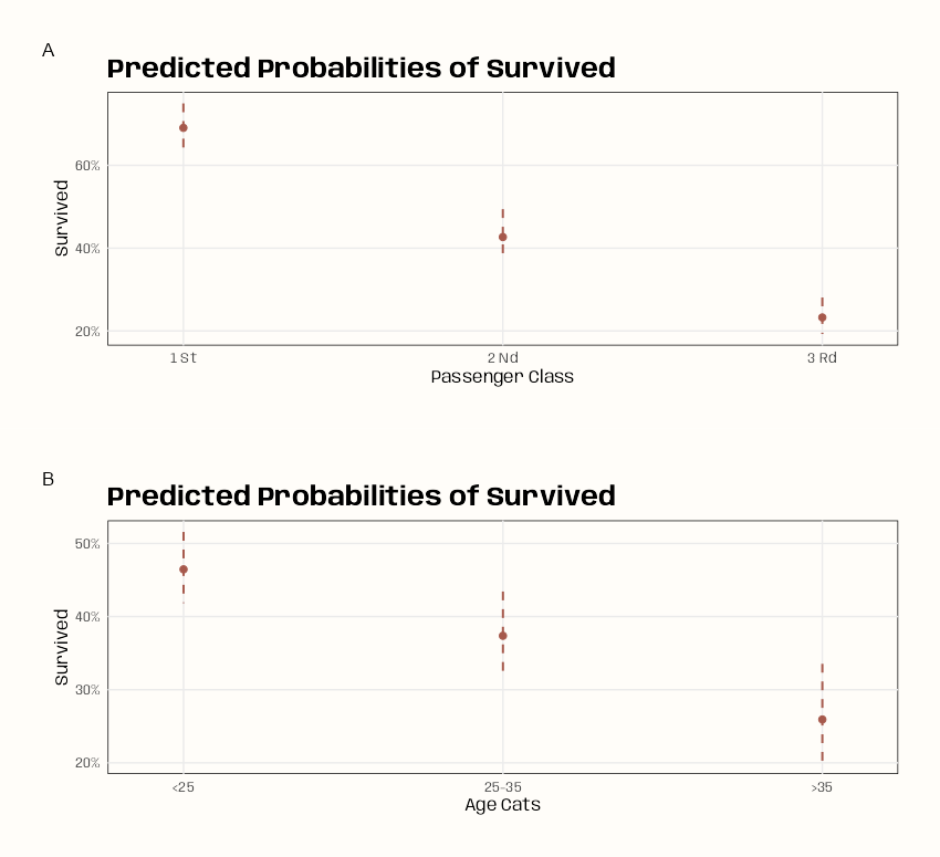
Marginal Means By Moderator
Binned Age, Balanced 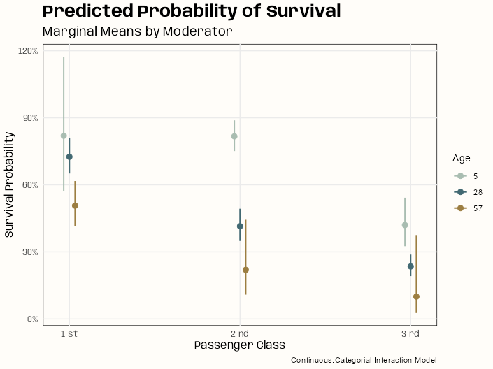
Splined Age, Centered Code
# categorical:categorial sjPlot::plot_model( m_bin_int_bal, type = "eff", terms = c("passengerClass", "age_cats"), colors = notebook_colors[c(2,6,7)], legend.title = "Age", title = "Predicted Probability of Survival" ) + labs(x = "Passenger Class", y = "Survival Probability", subtitle = "Marginal Means by Moderator", caption = "Categorical:Categorial Interaction Model") # continuous:categorial # backtransform centered age values leg_labels <- as.character(round(mean(d_cent$age) + c(-24.88, -1.88, 27.12)), 0) sjPlot::plot_model( m_spl_int_cent, type = "eff", terms = c("passengerClass", "age_cent [-24.88, -1.88, 27.12]"), legend.title = "Age", title = "Predicted Probability of Survival" ) + scale_color_manual(labels = leg_labels, values = notebook_colors[c(2,6,7)]) + labs(x = "Passenger Class", y = "Survival Probability", subtitle = "Marginal Means by Moderator", caption = "Continuous:Categorial Interaction Model")- For the spline model (continuous:categorical), a few of the point estimates have sizable uncertainty (SEs) associated with them. Since these are point estimates, there are probably few events for those ages in those passenger classes or it could be due to the collinearity that’s still present between the interaction and main effects terms (high VIFs).
- Quite a bit of overlap when the passenger class marginal means are broken down by age. The one group that sticks out in both models is the <25 age passengers in 2nd class. Both models’ charts indicate significance (much larger in the spline model) between this group and other ages in the same passenger class.
- Alternatively, {marginaleffects} has plotting functions which output {ggplot2} objects:
- Binned Age:
plot_predictions(m_bin_int_bal, by = c("passengerClass", "age_cats")) - Splined Age:
plot_predictions(m_spl_int_cent, condition = c("age_cent", "passengerClass"))- Order of variables matters. Putting age_cent first gets you the smooth on the X-axis.
- Binned Age:
Risk Ratio by Moderator
Code
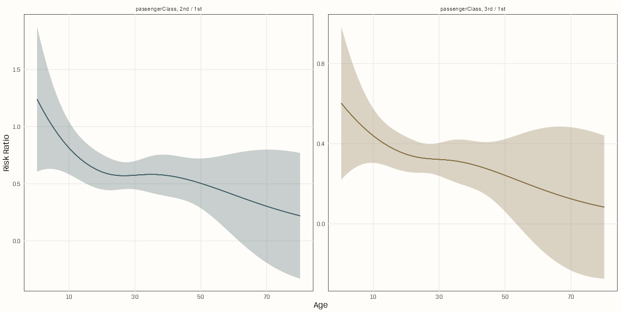
plot_comparisons(m_spl_int_cent, variables = "passengerClass", condition = "age_cent", comparison = "ratio") + scale_x_continuous(breaks = c(-20, 0, 20, 40), labels = xtick_labels) + geom_line(aes(y = estimate, x = .data[["age_cent"]], color = contrast)) + geom_ribbon(aes(y = estimate, x = .data[["age_cent"]], ymin = conf.low, ymax = conf.high, fill = contrast), alpha = 0.2) + scale_color_manual(values = notebook_colors[c(6,7)]) + scale_fill_manual(values = notebook_colors[c(6,7)]) + guides(color = "none", fill = "none") + labs(x = "Age", y = "Risk Ratio")- The
plot_*functions in {marginaleffects} output a ggplot object which allows you to perform theming and other styling options. It does not allow you style the points, line, ribbon, etc. which happen in thegeom(some stuff can be done using ggplot options). So the choices are either hack theplot_*object (see EDA, General >> Categorical Predictor vs Outcome >> Categorical Outcome >> Theseus Plot) or overwrite the geoms by repeating them. I chose the later here.- Save the
plot_*object to memory (i.e.moose <- plot_*) - Examine the object and look for the layers list element.
- Within each layer,
- the constructor element will show you the type of geom
- the mapping element will give you the variables in the mapping (ie.
aes)
- Repeat the necessary geoms with their mappings in your code, and add the desired styling arguments.
- In this case, I repeated
geom_lineandgeom_ribbon. By adding the color and fill arguments, I’m able to usescale_color_manualandscale_fill_manualto style of the line and ribbon.
- In this case, I repeated
- Save the
- Both risk ratios depend on age. As age of the passenger increases, the probability of survival for 1st class passengers increasingly surpasses those passengers of the same age in classes 2 and 3.
Slopes by Moderator
Code
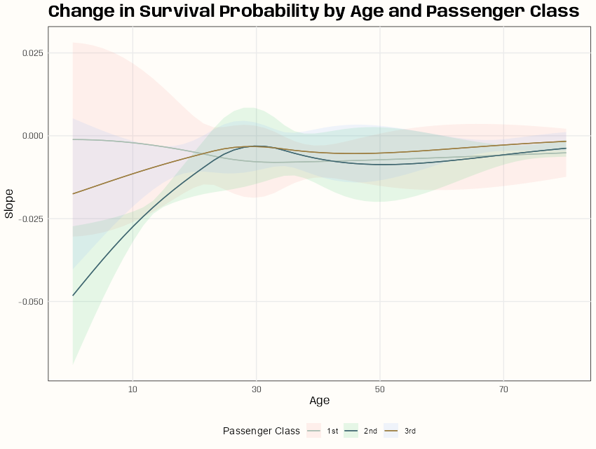
xtick_labels <- as.character(round(mean(d_cent$age) + c(-20, 0, 20, 40)), 0) plot_slopes(m_spl_int_cent, variables = "age_cent", condition = c("age_cent", "passengerClass")) + scale_x_continuous(breaks = c(-20, 0, 20, 40), labels = xtick_labels) + scale_color_manual(values = c("1st" = notebook_colors[[2]], "2nd" = notebook_colors[[6]], "3rd" = notebook_colors[[7]])) + labs(x = "Age", title = "Change in Survival Probability by Age and Passenger Class", color = "Passenger Class", fill = "Passenger Class") + theme(legend.position = "bottom")- variables is the variable whose slope will be on the Y-axis
- conditon is a vector or list of variables you want to stratify by
- The first variable listed will be on the X-axis, so you could, untraditionally have slope and x-axis variable be different.
- The second variable is a group by variable
- There seems to be some significant differences in slope under age 20 where an increase in age of passengers in class 2 and probably class 3 can have a negative effect on the probability of survival. Then, at about age 20 or 25, the differences in slopes converge until the slopes of all classes are almost 0.
Probit
- “For some reason, econometricians have never really taken on the benefits of the generalized linear modelling framework. So you are more likely to see an econometrician use a probit model than a logistic regression, for example. Probit models tended to go out of fashion in statistics after the GLM revolution prompted by Nelder and Wedderburn (1972).” (Hyndman)
- Very similar to Logistic

- Where probit and logistic curves differ

- link function: Φ-1(p) where Φ is the standard normal CDF:

- The probability prediction, p:

Starting Values
- GLM models that use non-standard link functions (e.g. Binomial w/log link, Poisson w/identitly link) sometimes require starting values in order to converge
glmhas a start argument that allows you to pass a vector of starting values- The values should be in the same order as the coefficients in the model (i.e. intercept is first, etc.)
- Number of Starting Values
- In a typical model, it should equal the number of coefficients + the intercept
- You can fit the model and then count the coefficients:
names(coef(mod)) - Example:
survived ~ passengerClass * age_cats- Where survived is a binary variable, passengerClass is a factor variable with 3 levels, age_cats is a factor variable with 3 levels.
- Number of Starting Values (Total of 9)
- Intercept: 1 parameter
- passengerClass: 2 parameters (3 levels - 1 reference level)
- age_cats: 2 parameters (3 levels - 1 reference level)
- Interaction (passengerClass:age_cats): 4 parameters (2 × 2 from the non-reference levels)
- Options
- Guidelines
- Values should be reasonable for your given link function
- e.g. With a log link, the values should be reasonable on the log scale
- Avoid extreme values that could cause numerical issues
- Values should be reasonable for your given link function
- Use zeros
- e.g.
start = rep(0, 9)
- e.g.
- Use estimates from the standard link model
Example:
# Fit logit model first
logit_model <-
  glm(survived ~ passengerClass * age_cats,
      data = d,
      family = binomial("logit"))
start_values <- coef(logit_model)

# Then use these as starting values for log model
log_model <-
  glm(survived ~ passengerClass * age_cats,
      data = d,
      family = binomial("log"),
      start = start_values)
- Data-informed values
Example
# Use overall survival rate
intercept_start <- log(mean(d$survived))

# Use small values for other parameters
start_values <- c(intercept_start, rep(0, 8))
- Slight perturbation around 0
- e.g.
start = rnorm(9, mean = 0, sd = 0.1)
- e.g.
- Guidelines
Visualization
Misc
- Notes from
- Packages
- {regress3d} - Plots regression surfaces and marginal effects in three dimensions.
- A multiple linear regression creates a flat regression surface. A multiple linear regression with an interaction term can be depicted as a curved regression surface with linear marginal effects.
- A generalized linear model (glm) takes a linear component as a variable in a nonlinear function, creating a curved regression surface with nonlinear marginal effects.
- {regress3d} - Plots regression surfaces and marginal effects in three dimensions.
- Tables
.png)
- Appropriate for technical audiences who are familiar with logistic regression
- Can be taxing on the eyes making it difficult to absorb insights from your model
Log Odds Ratio vs Odds Ratio
.png)
- Using log odds ratio is recommended for visualizations for puposes of comparing effect magnitudes
- Each coefficient represents an additive change on the log odds scale; when we exponentiate to get odds, each coefficient represents a multiplicative change
- Odds ratios makes the chart asymmetric and squishes some bars (e.g. Pet: Fish)
- Odds ratios can be misleading in comparing negative vs postive variable effects
- e.g. Prior GPA looks like it has much bigger effect than Pet: Fish when using odds ratio
- There’s a danger that the percent change in odds might be misinterpreted as the absolute probability of the outcome (or the change in its probability)
- e.g. A 300% change in the odds ratio is a tripling of the odds ratio, not an 300% increase in probability. (see example below)
- Although numerically, changes in odds ratios may be a bit easier to describe for your audience than changes in log odds.
- Example: tripling the odds ratio is like going from 3-to-1 odds to 9-to-1 odds, or from 1-to-3 odds to an even chance.)
- Using log odds ratio is recommended for visualizations for puposes of comparing effect magnitudes
Error bar chart (caterpillar chart)
- Change in log odds
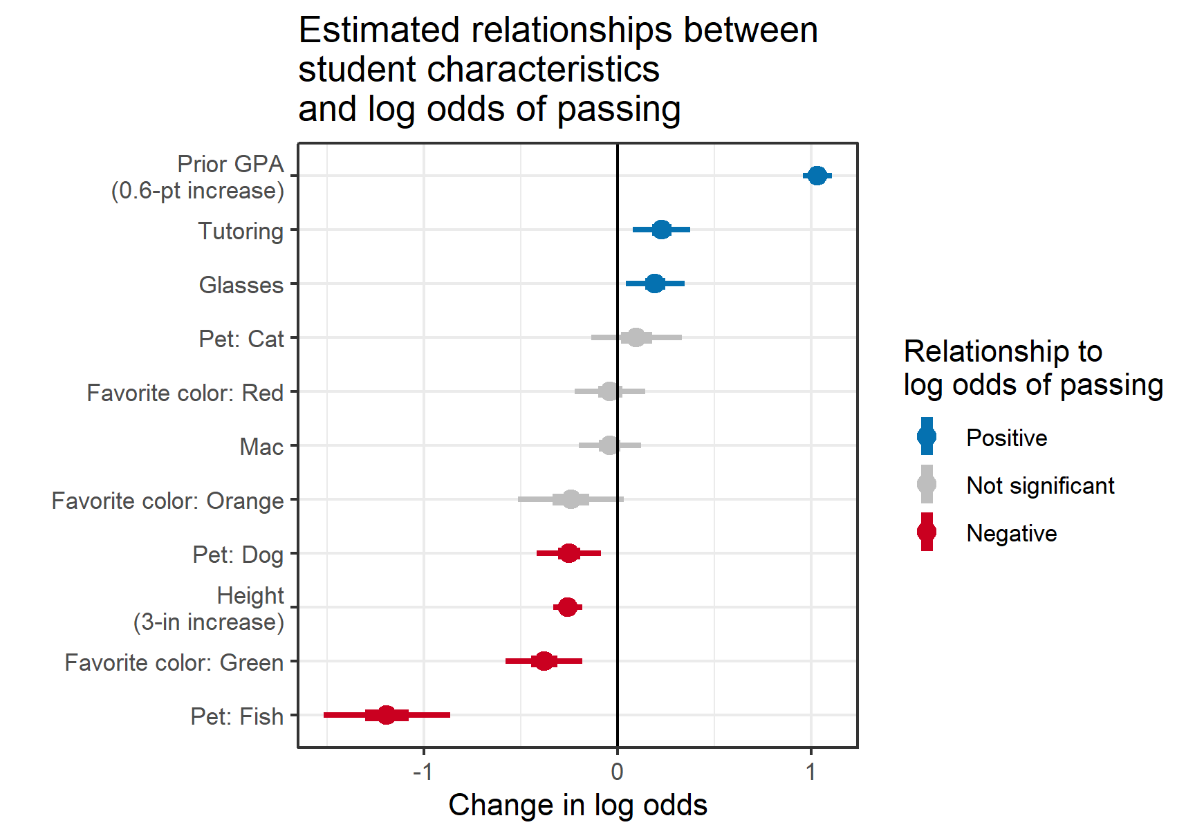
- These are untransformed parameter estimates (See Misc >> Tables for estimate values)
- Change in probability from a baseline
- Since the effect is non-linear (See Interpetation >> Effect is non-linear in p), a baseline is needed in order to properly interpret the changes in probability due to the increases of 1 unit of a variable
- Process:
- Choose an appropriate baseline
- Compute the marginal effect of a predictor given that baseline
- Intercept as a baseline
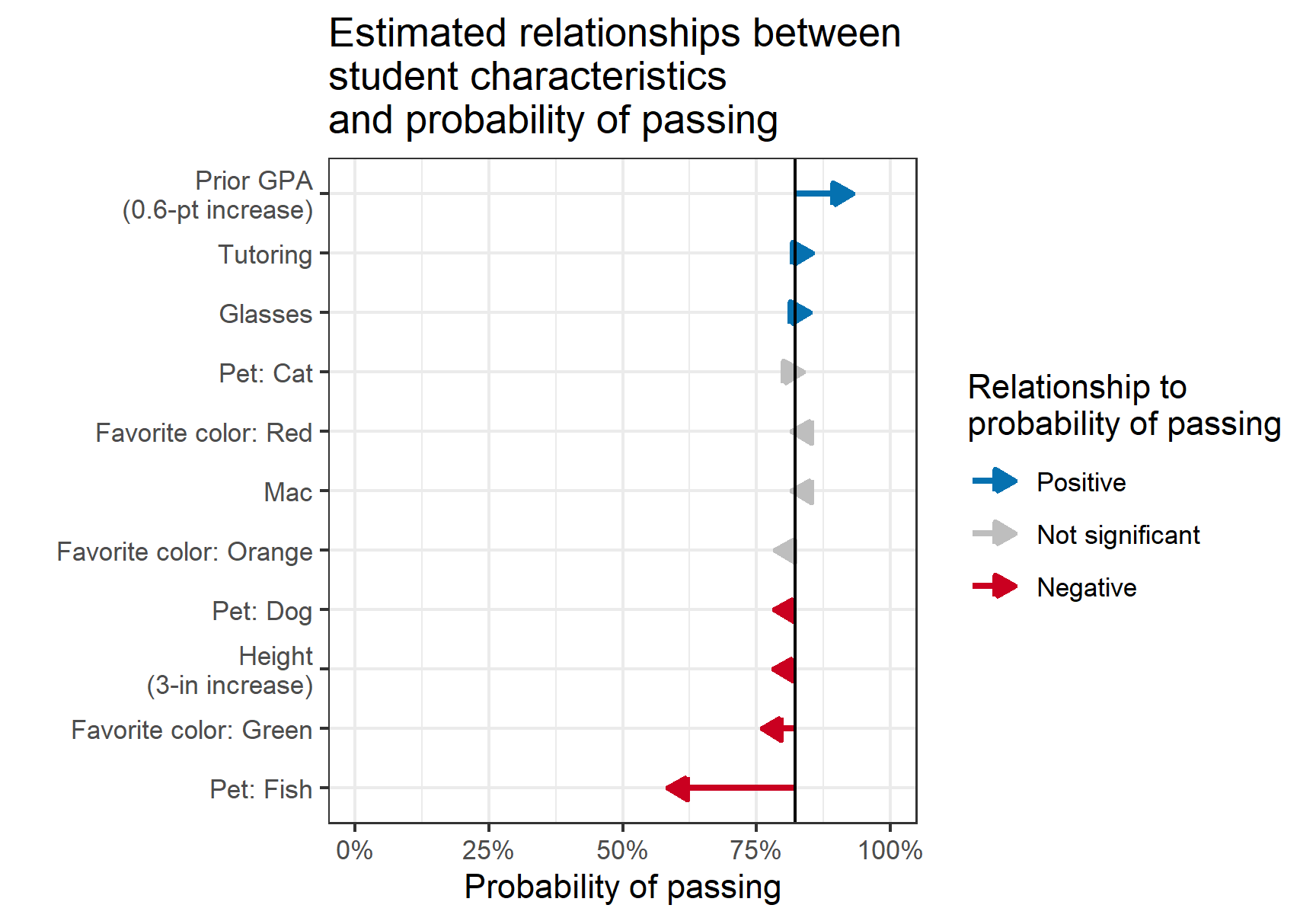
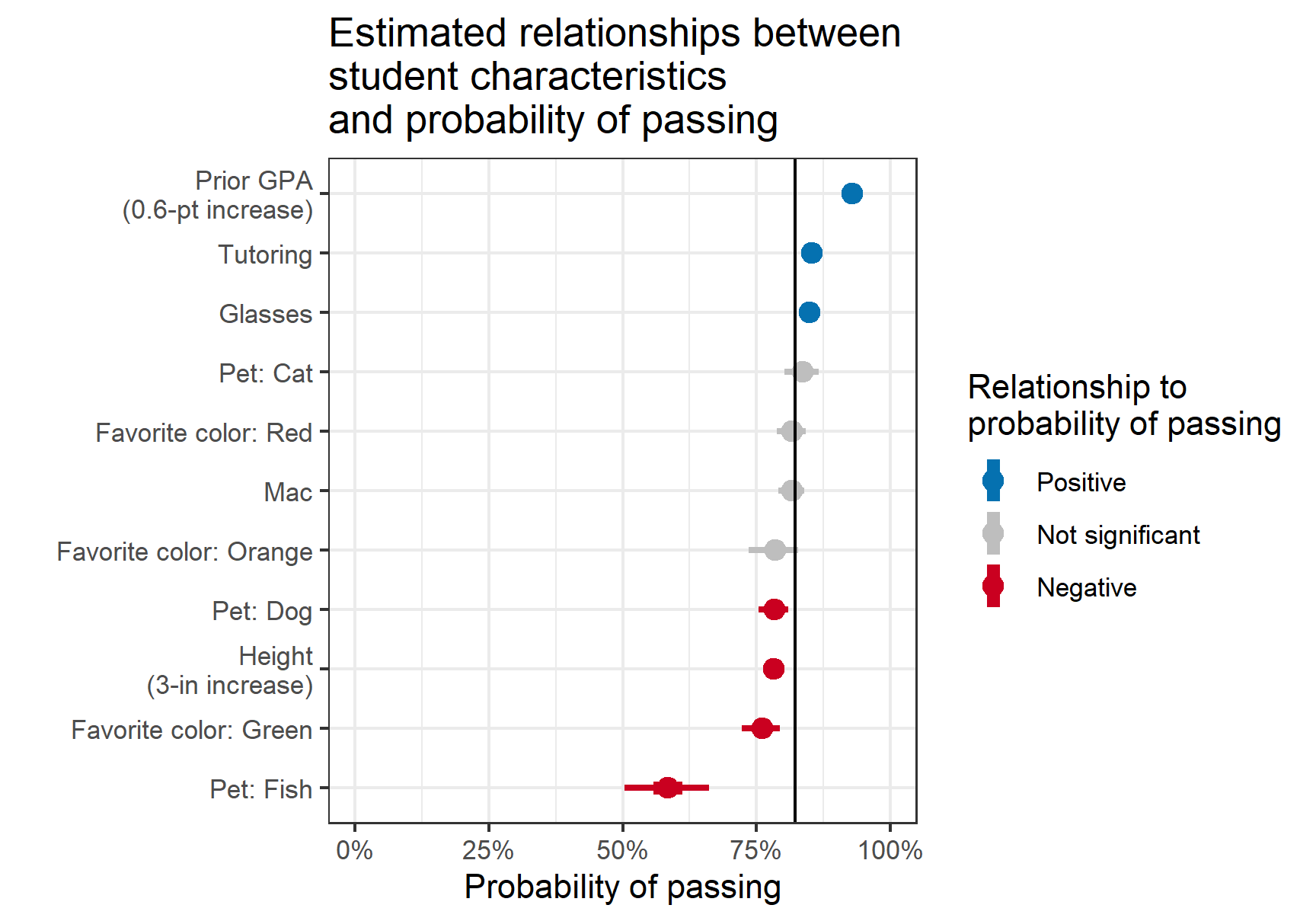
- The x-axis is the problem. Values shown depict changes from the baseline
- Both charts have the same values, but the chart on the left more clearly indicates the meaning while the chart on the right includes the CIs
- Estimates transformations
- Intercept:
invlogit(intercept) - Other parameters:
invlogit(<param> + intercept)- Including CI values
- Intercept:
- Vertical line is the output of the inverse logit of the intercept
- Representing the probability of passing for a student with average prior GPA, average height, and the baseline value of each categorical variable – not a Mac user, doesn’t wear glasses, has no pet, favorite color is blue, and didn’t go to tutoring.
- Change in log odds
Outcome vs Predictor with Logistic Curve
Example 1:
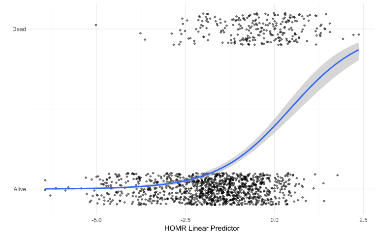
# Plot of data with a logistic curve fit ggplot(data, aes(x = z_homr, y = as.numeric(alive) - 1)) + geom_jitter(height = 0.1, size =1, alpha = 0.5) + geom_smooth(method = "glm", method.args = list(family = "binomial")) + theme_minimal() + scale_y_continuous(breaks = c(0, 1), labels = c("Alive", "Dead")) + ylab("") + xlab("HOMR Linear Predictor")- Dead/Alive is the outcome and HOMR is the predictor
Example 2: (source)
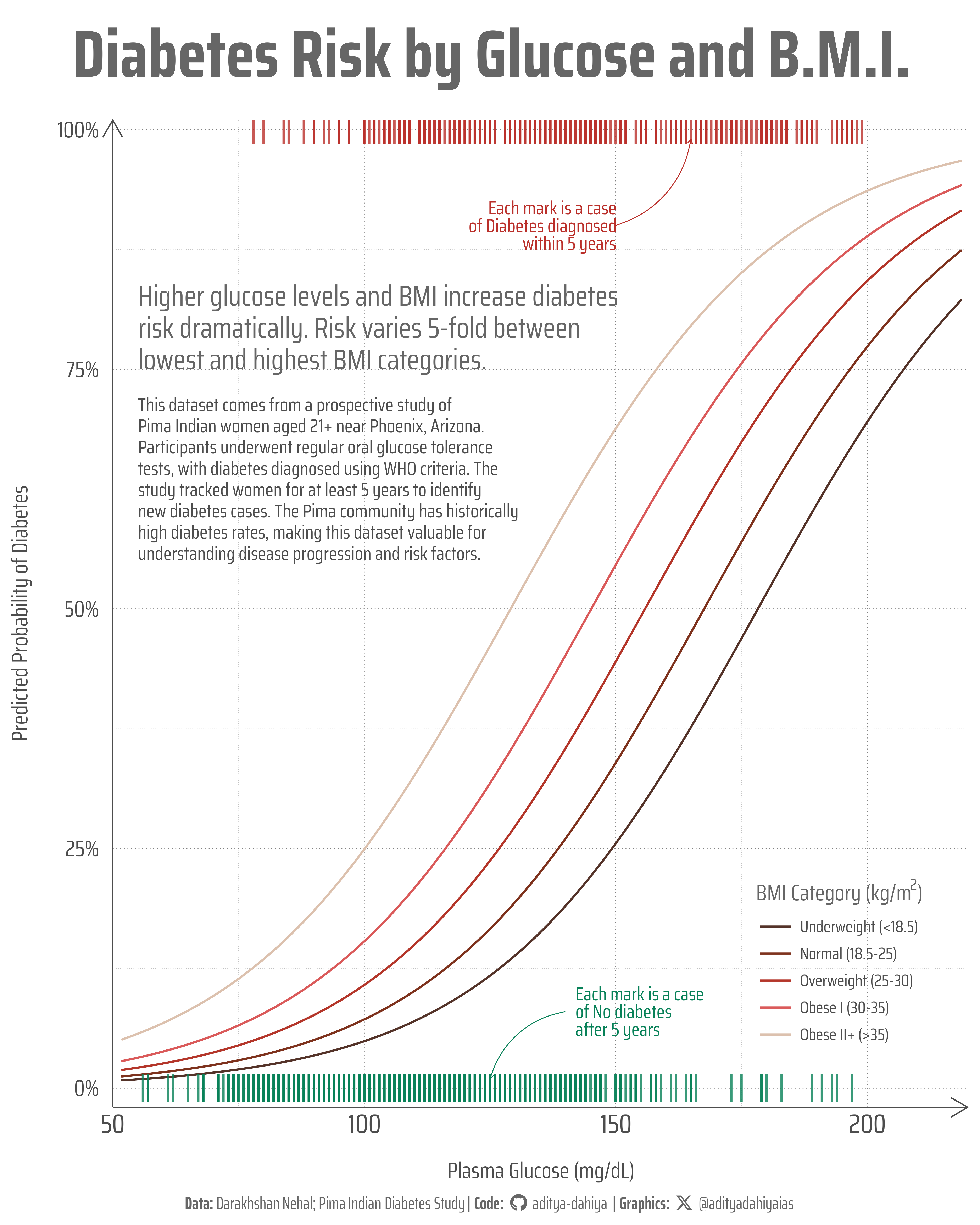
Predictor by outcome (count)
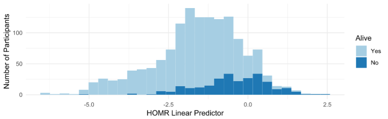
g1 <- ggplot(data, aes(x = z_homr, fill = alive)) +
    geom_histogram() +
    theme_minimal() +
    xlab("HOMR Linear Predictor") +
    ylab("Number of Participants") +
    scale_fill_brewer("Alive", palette = "Paired")
Predictor by outcome (proportion)
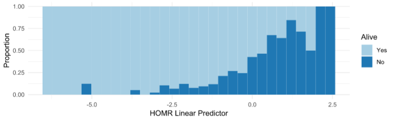
g2 <- ggplot(data, aes(x = z_homr, fill = alive)) +
    geom_histogram(position = "fill") +
    theme_minimal() +
    xlab("HOMR Linear Predictor") +
    ylab("Proportion") +
    scale_fill_brewer("Alive", palette = "Paired")
Predictor vs Outcome (beeswarm)
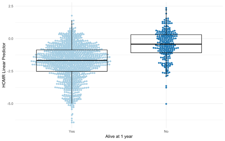
ggplot(data, aes(y = z_homr, x = alive, fill = alive, color = alive)) +
    geom_beeswarm() +
    geom_boxplot(alpha = 0, color = "black") +
    theme_minimal() +
    ylab("HOMR Linear Predictor") +
    xlab("Alive at 1 year") +
    scale_fill_brewer(guide = FALSE, palette = "Paired") +
    scale_color_brewer(guide = FALSE, palette = "Paired")