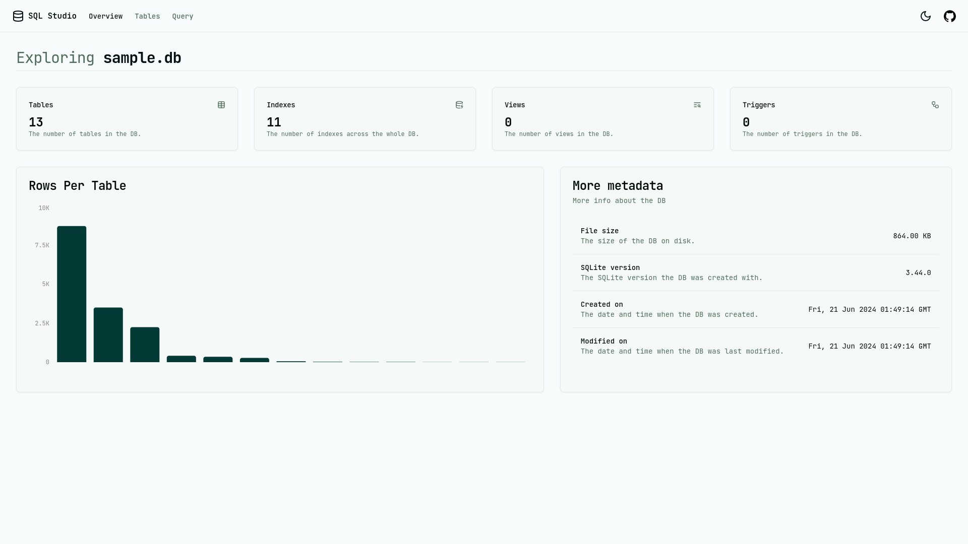
SQL
Misc
Resources
- Publicly Available SQL Databases: Need to email administrator to gain access
- SQL for Data Scientists in 100 Queries
- SQLite, administrative commands, query commands, JSON ops, python
For WSL/linux users, if installing odbc for R via
install.packages('odbc')throws an error, try installing unixodbc in a bash terminal,sudo apt install unixodbc(source)dplyr::show_querycan convert a dplyr expression to SQL for db object (e.g. dbplyr, duckdb, arrow)Queries in examples
- Window Functions
- Average Salary by Job Title
- Average Unit Price for each CustomerId
- Rank customers by amount spent
- Create a new column that ranks Unit Price in descending order for each CustomerId
- Create a new column that provides the previous order date’s Quantity for each ProductId
- Create a new column that provides the very first Quantity ever ordered for each ProductId
- Calculate a cumulative moving average UnitPrice for each CustomerId
- Rank customers for each department by amount spent
- Find the model and year of the car that been on the lot the longest
- Create a subset (CTE)
- Calculate a running monthly total (aka cumsum)
- Also running average
- Calculate a running monthly total for each account id
- Calculate a 3 months rolling running total using a window that includes the current month.
- Calculate a 7 months rolling running total using a window where the current month is always the middle month
- Calculate the number of consecutive days spent in each country
- Calculate a running monthly total (aka cumsum)
- Three-day moving average of the temperature in each city
- CTE
- Average monthly cost per campaign for the company’s marketing efforts
- Count the number of interactions of new users
- The average top Math test score for students in California
- Business Queries
- Total Sales, Customers, Sales per Customer per Region
- 7-day Simple Moving Average (SMA)
- Rank product categories by shipping cost for each shipping address
- Total order quantity for each month
- Monthly and yearly total orders and average shipping costs
- Daily counts of open jobs (where “open” is an untracked daily status)
- Get the latest order from each customer
- Overall median price
- Median price for each product
- Overall median price and quantity
- Processing Expressions
- Provide subtotals for a hierarchical group of fields (e.g. family, category, subcategory)
- See NULLs >> COALESCE
- Provide subtotals for a hierarchical group of fields (e.g. family, category, subcategory)
- Window Functions
Order of Operations
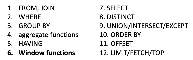
- Higher ranked functions can be inserted inside lower ranked functions
- e.g a window function can be inside a SELECT function but not inside a WHERE clause
- There are exceptions and hacks around this in some cases
- Higher ranked functions can be inserted inside lower ranked functions
Types of Commands
- Data Query Language (DQL) - used to find and view data without making any permanent changes to the database.
- Data Manipulation Language (DML) - used to make permanent changes to the data, such as updating values or deleting them.
- Data Definition Language (DDL) - used to make permanent changes to the table, such as creating or deleting a table.
- Data Control Language (DCL) - used for administrative commands, such as adding or removing users of different tables and databases.
- Transact Control Language (TCL) - advanced SQL that deals with transaction level statements.
Microsoft SQL Server format for referencing a table:
[database].[schema].[tablename]
Alternative
USE my_data_base
GO
Set-up
- postgres
- Download postgres
- pgAdmin is an IDE commonly used with postgres
- Open pgAdmin and click on “Add new server.”
- Sets up connection to existing server so make sure postgres is installed beforehand
- Create Tables
- home >> Databases (1) >> postgres >> Query Tool
- If needed, give permission to pgAdmin to access data from a folder
- Might be necessary to upload csv files
- Import csv file
- right-click the table name >> Import/Export
- Options tab
- Select import, add file path to File Name, choose csv for format, select Yes for Header, add , for Delimiter
- Columns tab
- uncheck columns not in the csv (probably the primary key)
- Wonder if NULLs will be automatically inserted for columns in the table that aren’t in the file.
- uncheck columns not in the csv (probably the primary key)
- Open pgAdmin and click on “Add new server.”
- psql - PostgreSQL interactive terminal. Allows you to script and automate tasks, e.g. tests, check errors, and do data entry on the command line.
- Cheatsheet
- Requires
- The user name and password for your PostgreSQL database
- The IP address of your remote instance if working remotely
- The db=# prompt indicates the command line interface (CLI) prompt. Here’s a breakdown of what each part means:
- db: This is the name of the current database to which you are connected.
- =#: This is the prompt symbol that appears when you are logged in as a superuser (like postgres). If you were logged in as a regular user, the prompt would be =>
- Example:
Input
db=# CREATE TABLE tags (
  id INT GENERATED BY DEFAULT AS IDENTITY PRIMARY KEY,
  name VARCHAR(50) NOT NULL
);
Output
CREATE TABLE- The way psql indicates the command was successful is by confusingly printing the command.
Terms
- Batch - a set of sql statements e.g. statements between BEGIN and END
- Compiled object - you can create a function written in C/C++ and load into the database (at least in postgres) to achieve high performance.
- Correlated Columns - tells how good the match between logical and physical ordering is.
- Correlated/Uncorrelated Subqueries
correlated- a type of query, where inner query depends upon the outcome of the outer query in order to perform its execution
- A correlated subquery can be thought of as a filter on the table that it refers to, as if the subquery were evaluated on each row of the table in the outer query
- A correlated subquery can be thought of as a filter on the table that it refers to, as if the subquery were evaluated on each row of the table in the outer query
uncorrelated - a type of sub-query where inner query doesn’t depend upon the outer query for its execution.
- It is an independent query, the results of which are returned to and used by the outer query once (not per row).
-- Uncorrelated subquery:
-- inner query, c1, only depends on table2
select c1, c2
  from table1 where c1 = (select max(x) from table2);

-- Correlated subquery:
-- inner query, c1, depends on table1 and table2
select c1, c2
  from table1 where c1 = (select x from table2 where y = table1.c2);
- Functions - Execute at a different level of priority and are handled differently than Views. You will likely see better performance.
- Idempotent - Providing the same input should always produce the same output, e.g. A plain
INSERTis not idempotent because executing the command with the same input for the second time will trigger an error. - Index - A quick lookup table (e.g. field or set of fields) for finding records users need to search frequently. An index is small, fast, and optimized for quick lookups. It is very useful for connecting the relational tables and searching large tables. (also see DB, Engineering >> Cost Optimizations)
- Migrations (schema) - A version control system for your database schema. Management of incremental, reversible changes and version control to relational database schemas. A schema migration is performed on a database whenever it is necessary to update or revert that database’s schema to some newer or older version.
- Physical Ordering - A PostgreSQL table consists of one or more files of 8KB blocks (or “pages”). The order in which the rows are stored in the file is the physical ordering.
- Predicate - Defines a logical condition being applied to rows in a table. (e.g. IN, EXISTS, BETWEEEN, LIKE, ALL, ANY)
- Scalar/Non-Scalar Subqueries
- A scalar subquery returns a single value (one column of one row). If no rows qualify to be returned, the subquery returns NULL.
- A non-scalar subquery returns 0, 1, or multiple rows, each of which may contain 1 or multiple columns. For each column, if there is no value to return, the subquery returns NULL. If no rows qualify to be returned, the subquery returns 0 rows (not NULLs).
- Selectivity - The fraction of rows in a table or partition that is chosen by the predicate
- Refers to the quality of a filter in its ability to reduce the number of rows that will need to be examined and ultimately returned
- With a high selectivity, using the primary key or indexes to get right to the rows of interest
- With a low selectivity, a full table scan would likely be needed to get the rows of interest.
- Higher selectivity means: more unique data; fewer duplicates; fewer number of rows for each key value
- Used to estimate the cost of a particular access method; it is also used to determine the optimal join order. A poor choice of join order by the optimizer could result in a very expensive execution plan.
- Refers to the quality of a filter in its ability to reduce the number of rows that will need to be examined and ultimately returned
- Soft-deleted - An operation in which a flag is used to mark data as unusable, without erasing the data itself from the database
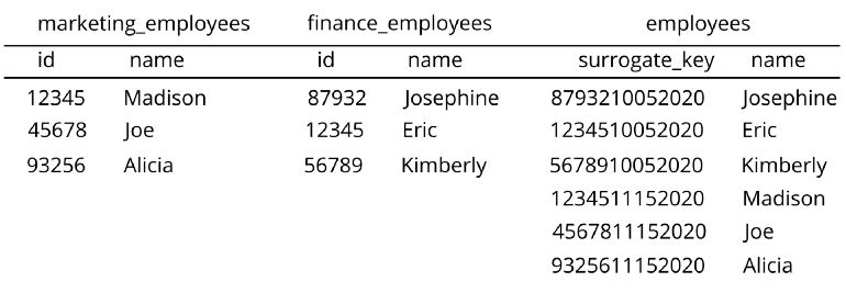
- Surrogate key - Very similar to a primary key in that it is a unique value for an object in a table. However, rather than being derived from actual data present in the table, it is a field generated by the object itself. It has no business value like a primary key does, but is rather only used for data analysis purposes. Can be generated using different columns that already exist in your table or more often from two or more tables. dbt function definition
- Examples: PostgreSQL serial column, Oracle sequence column, or MySQL auto_increment column, Snowflake _file + _line columns
- Example: Each employee id is concatenated with a department id (e.g. marketing or finance)
- Transaction - A set of queries tied together such that if one query fails, the entire set of queries are rolled back to a pre-query state if the situation dictates.
- A database transaction, by definition, must be atomic, consistent, isolated and durable. These are popularly known as ACID properties. These properties can ensure the concurrent execution of multiple transactions without conflict.
- Views - Database objects that represent saved SELECT queries in “virtual” tables.
- Contains a query plan. For each query executed, the planner has to evaluate what’s being asked and calculate an optimal path. Views already have this plan calculated so it allows subsequent queries to be returned with almost no friction in processing aside from data retrieval.
- Some views are updateable but under certain conditions (1-1 mapping of rows in view to underlying table, no group_by, etc.)
Basics
Misc
DROP TABLE <table name>- Deletes table from database. Used to remove obsolete or redundant tables from the database.- Comments
Single Line
-- Select all: SELECT * FROM Customers; SELECT * FROM Customers -- WHERE City='Berlin';- Any text between
--and the end of the line will be ignored (will not be executed)
- Any text between
Multi-Line
/*Select all the columns
of all the records
in the Customers table:*/
SELECT * FROM Customers;
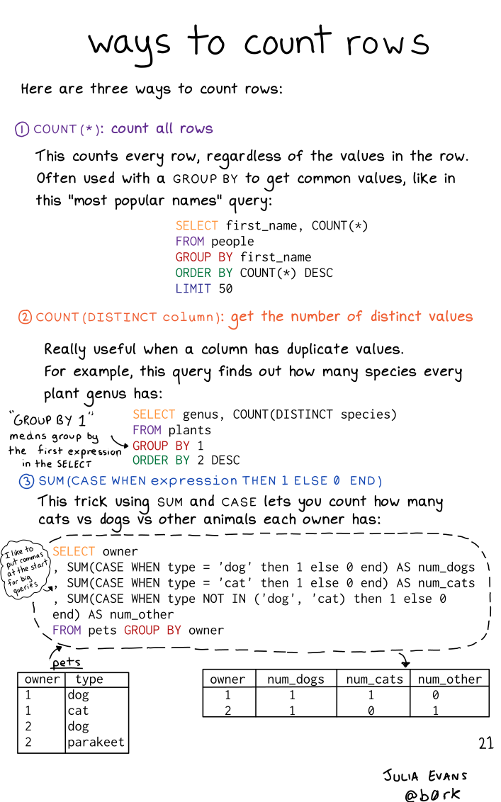
- Counting Rows
Create Tables
If you don’t include the schema as part of the table name (e.g. schema_name.table_name), pgadmin automatically places it into the “public” schema directory
Field Syntax: name, data type, constraints
Example: Create table as select (CTAS)
CREATE TABLE new_table AS SELECT * FROM old_table WHERE condition;Example: Table 1 (w/primary key)
DROP TABLE IF EXISTS classrooms CASCADE;
CREATE TABLE classrooms (
    id INT PRIMARY KEY GENERATED ALWAYS AS IDENTITY,
    teacher VARCHAR(100)
    );
 -- OR
CREATE TABLE classrooms (
    id INT GENERATED ALWAYS AS IDENTITY,
    teacher VARCHAR(100)
    PRIMARY KEY(id)
    );
“classrooms” is the name of the table; “id” and “teacher” are the fields
CASCADE- postgres won’t delete the table if other tables point to it, so cascade will override measure.GENERATED ALWAYS AS IDENTITY- makes it so you don’t have to keep track of which “id” values have been used when adding rows. You can ommit the value for “id” and just add the values for the other fields- Also seen
id INT GENERATED BY DEFAULT AS IDENTITY PRIMARY KEY
- Also seen
See tutorial for options, usage, removing, adding, etc. this constraint
INSERT INTO classrooms (teacher) VALUES ('Mary'), ('Jonah');- Also see Add Data >> Example: chatGPT
Example: Table 2 (w/foreign key)
DROP TABLE IF EXISTS students CASCADE; CREATE TABLE students ( id INT PRIMARY KEY GENERATED ALWAYS AS IDENTITY, name VARCHAR(100), classroom_id INT, CONSTRAINT fk_classrooms FOREIGN KEY(classroom_id) REFERENCES classrooms(id) );- “students” is the name of the table; “id”, “name”, and “classroom_id” are the fields
- Create a foreign key that points to the “classrooms” table
Expression
- fk_classrooms is the name of the
CONSTRAINT - “classroom_id” is the field that will be the
FOREIGN KEY REFERENCESpoints the foreign key to the classrooms table’s primary key, “id”- foreign keys can point to any table
- fk_classrooms is the name of the
Postgres won’t allow you to insert a row into students with a “classroom_id” that doesn’t exist in the “id” field of classrooms but will allow you to use a NULL placeholder
-- Explicitly specify NULL INSERT INTO students (name, classroom_id) VALUES ('Dina', NULL); -- Implicitly specify NULL INSERT INTO students (name) VALUES ('Evan');- Also see Add Data >> Example: chatGPT
Example
CREATE TABLE members ( id serial primary key, second_name character varying(200) NOT NULL, date_joined date NOT NULL DEFAULT current_date, member_id integer references members(id), booking_start_time timestamp without timezone NOT NULL- The “serial” data type does the same thing as
GENERATED ALWAYS AS IDENTITY(see first example), but is NOT compliant with the SQL standard. UseGENERATED ALWAYS AS IDENTITY - “references” seems to be another old way to create foreign keys (see 2nd example for proper way)
- “character varying” - variable-length with limit (e.g limit of 200 characters)
- character(n), char(n) are for fixed character lengths; text is for unlimited character lengths
- “current_date” is a function that will insert the current date as a value
- “timestamp without timezone” is literally that
- also available: time with/without timezone, date, interval (see Docs for details)
- The “serial” data type does the same thing as
Example: MySQL
CREATE DATABASE products;

CREATE TABLE `products`.`prices` (
  `pid` int(11) NOT NULL AUTO_INCREMENT,
  `category` varchar(100) NOT NULL,
  `price` float NOT NULL,
  PRIMARY KEY (`pid`)
);

INSERT INTO products.prices
    (pid, category, price)
VALUES
    (1, 'A', 2),
    (2, 'A', 1),
    (3, 'A', 5),
    (4, 'A', 4),
    (5, 'A', 3),
    (6, 'B', 6),
    (7, 'B', 4),
    (8, 'B', 3),
    (9, 'B', 5),
    (10, 'B', 2),
    (11, 'B', 1)
;
Add Data
Example: Add data via .csv
COPY assignments(category, name, due_date, weight) FROM 'C:/Users/mgsosna/Desktop/db_data/assignments.csv' DELIMITER ',' CSV HEADER;- assignments is the table; [category][assignments], [name][assignments], [due_date][assignments], [weight][assignments] are fields that you want to import from the csv file
- ** The order of the columns must be the same as the ones in the CSV file **
HEADERkeyword to indicate that the CSV file contains a header- Might need to have superuser access in order to execute the
COPYstatement successfully
Update Table
Resources
- How to Get or Create in PostgreSQL
- Deep dive on using
INSERTandMERGE
- Deep dive on using
- How to Get or Create in PostgreSQL
Check if a table is updatable
SELECT table_name, is_updatable FROM information_schema.views- Useful if some of the tables you are working with are missing values that you need to add
- If not updatable, then you’ll need to contact the database administrator to request permission to update that specific table
Update target table by transaction id (BQ)(link)
insert target_table (transaction_id) select transaction_id from source_table where transaction_id > (select max(transaction_id) from target_table) ;- Might not be possible with denormalized star-schema datasets in modern data warehouses.
Update Target Table by transaction date (BQ) (link)
merge last_online t using ( select user_id, last_online from ( select user_id, max(timestamp) as last_online from connection_data where date(_partitiontime) >= date_sub(current_date(), interval 1 day) group by user_id ) y ) s on t.user_id = s.user_id when matched then update set last_online = s.last_online, user_id = s.user_id when not matched then insert (last_online, user_id) values (last_online, user_id) ; select * from last_online ;MERGEperformsUPDATE,DELETE, andINSERT- UPDATE or DELETE clause can be used when two or more data match.
- INSERT clause can be used when two or more data are different and do not match.
- The UPDATE or DELETE clause can also be used when the given data does not match the source.
- _partitiontime is a field BQ creates to record the row’s ingestion time (See Databases, BigQuery >> Optimization >> Partitions
Update Target Table with Source Data (link)
MERGE INTO target_table tgt USING source_table src ON tgt.customer_id = src.customer_id WHEN MATCHED THEN UPDATE SET tgt.is_active = src.is_active, tgt.updated_date = '2024-04-01'::DATE WHEN NOT MATCHED THEN INSERT (customer_id, is_active, updated_date) VALUES (src.customer_id, src.is_active, '2024-04-01'::DATE) ;- The statement uses the
MERGEkeyword to conditionally update or insert rows into a target table based on a source table. - It matches rows between the tables using the
ONclause and thecustomer_idcolumn. - The
WHEN MATCHED THENclause specifies the update actions for matching rows. - The
WHEN NOT MATCHED THENclause specifies the insert actions for rows that don’t have a match in the target table. - The
::DATEcast ensures that theupdated_datevalue is treated as a date.
- The statement uses the
Delete Rows
- Misc
- Be cautious when using CTEs with
DELETE(orUPDATE) andLIMIT, especially when relying on theRETURNINGclause for atomicity. The planner’s optimization choices might surprise you and lead to behavior counter to your intent (e.g. unnecessary loops).
- Be cautious when using CTEs with
- DELETE FROM
Example: postgres (source)
DELETE FROM task_queue WHERE id = ( SELECT id FROM task_queue WHERE queue_group_id = 15 LIMIT 1 FOR UPDATE SKIP LOCKED ) RETURNING item_id; ) SELECT item_id FROM deleted_tasks;- Find one available task row (
LIMIT 1), delete it, and return its associateditem_id. - Use
WHERE id =for a single expected ID - If you strictly need to handle the case where zero rows might be found by the subquery without erroring, using
id IN (...)might be necessary.- Make sure to test the plan, because the planner has been known to choose a less efficient loop plan where the subquery gets ran more than once.
- Find one available task row (
DELETE CASCADEDeletes related rows in child tables when a parent row is deleted from the parent table
Apply cascade to foreign key in the child table
CREATE TABLE parent_table(
    id SERIAL PRIMARY KEY,
    ...
);

CREATE TABLE child_table(
    id SERIAL PRIMARY KEY,
    parent_id INT,
    FOREIGN_KEY(parent_id)
       REFERENCES parent_table(id)
       ON DELETE CASCADE
);
In the child table, the parent_id is a foreign key that references the id column of the parent_table.
The
ON DELETE CASCADEis the action on the foreign key that will automatically delete the rows from the child_table whenever corresponding rows from the parent_table are deleted.Example
DELETE FROM parent_table WHERE id = 1;- id = 1 in parent_table corresponds to parent_id = 1 in child_table. Therefore, all rows matching those conditions in both tables will be deleted.
Subqueries
**Using CTEs instead of subqueries make code more readable**
- Subqueries make it difficult to understand their context in the larger query
- The only way to debug a subquery is by turning it into a CTE or pulling it out of the query entirely.
- CTEs and subqueries have a similar runtime, but subqueries make your code more complex for no reason.
Notes from How to Use SubQueries in SQL
- Also shows the alt method of creating a temporary table to compute the queries
Use cases
- Filtering rows from a table with the context of another.
- Performing double-layer aggregations such as average of averages or an average of sums.
- Accessing aggregations with a subquery.
Tables used in examples
- Store A (store_a)
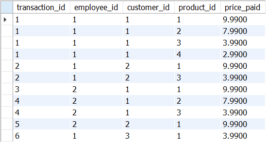
- Store B is similar
- Store A (store_a)
Example: Filtering rows
select * from sandbox.store_b where product_id IN ( select product_id from sandbox.store_b group by product_id having count(product_id) >= 3 );- filters the rows with products that have been bought at least three times in store_b
Example: Multi-Layer Aggregation
select avg(average_price.total_value) as average_transaction from ( select transaction_id, sum(price_paid) as total_value from sandbox.store_a group by transaction_id ) as average_price ;- computes the average of all transactions
- can’t apply an average directly, as our table is oriented to product_ids and not to transaction_ids
Example: Filtering the table based on an Aggregation
select @avg_transaction:= avg(agg_table.total_value) from ( select transaction_id, sum(price_paid) as total_value from sandbox.store_a group by transaction_id ) as agg_table; select * from sandbox.store_a where transaction_id in ( select transaction_id from sandbox.store_a group by transaction_id having sum(price_paid) > @avg_transaction )- filters transactions that have a value higher than the average (where the output must retain the original product-oriented row)
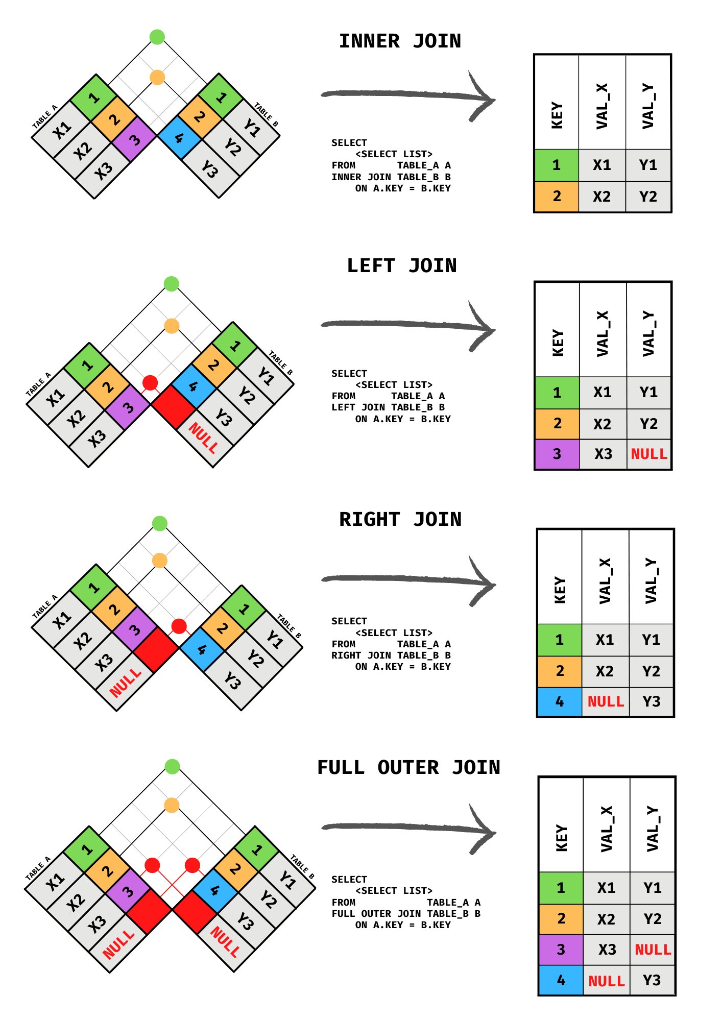
Joins
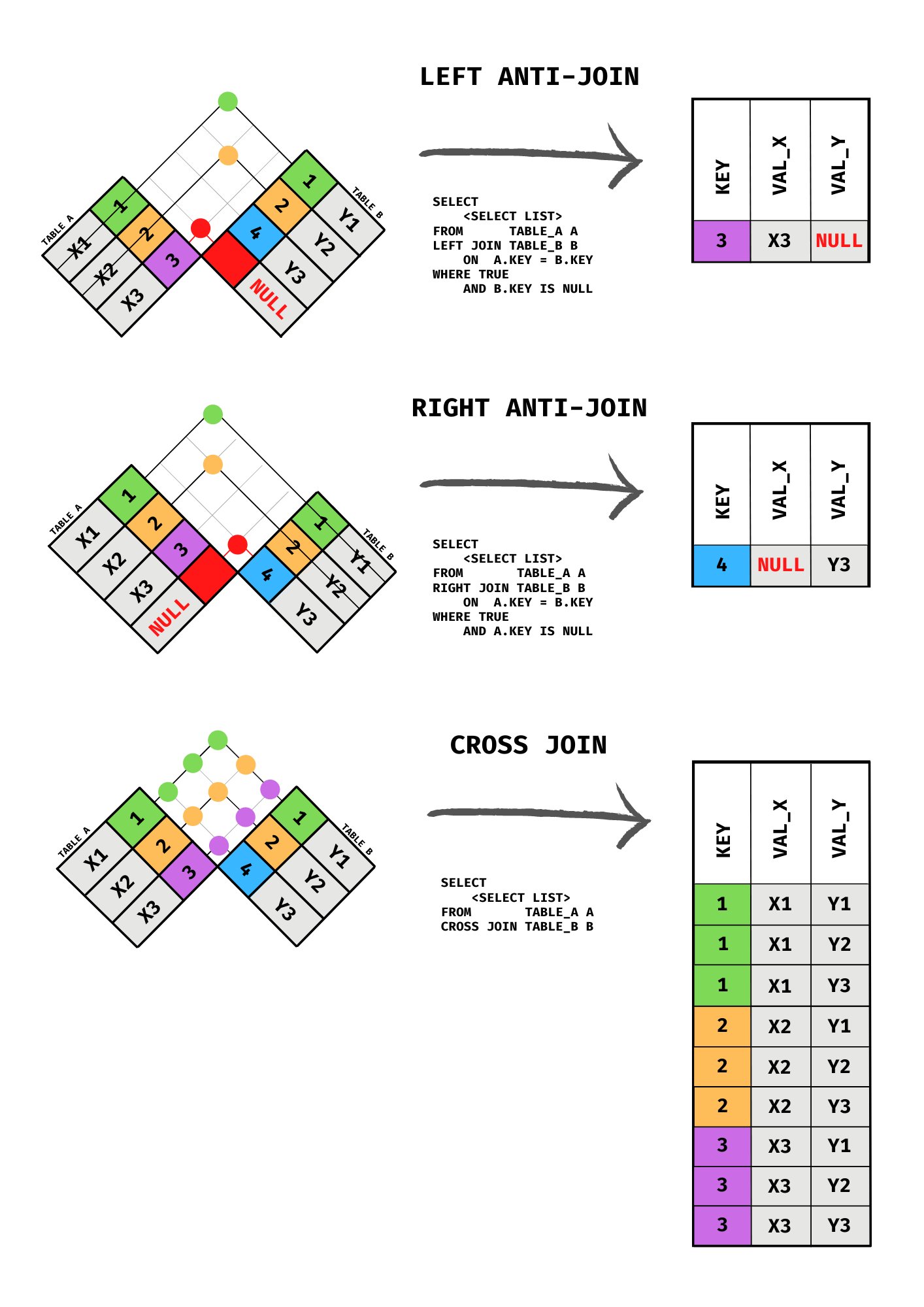
Cross Join - acts like an expand_grid; where each value in the join key column gets all combinations of rows in both tables (also see above pic)
Efficient join
When you add the
whereclause, the cross join acts similarly to aninner join, except you aren’t joining it on any specified columnExample:
SELECT schedule.event, calendar.number_of_days FROM schedule CROSS JOIN calendar WHERE schedule.total_number < calendar.number_of_days- Only join the row in the “schedule” table with the rows in the “calendar” table that meet the specified condition
Natural Join - don’t need to specify join columns; need to have two columns in each table with the same name
- Use cases
- There are a lot of common columns with the same name across multiple tables
- They will all be used as joining keys.
- You don’t want to type out all of the common columns in select just to avoid outputting the same columns multiple times.
- There are a lot of common columns with the same name across multiple tables
select * from table_a natural join table_b ; -- natural + outer select * from table_a natural outer join table_b ;- Use cases
R
Misc
- Thread regarding querying when permissions/privileges only allow partial access to a table (e.g. specific columns)
- Packages
- {dbi.table} - Database Queries Using ‘data.table’ Syntax
- {SQLFormatteR} - Provides an easy-to-use wrapper for the sqlformat-rs Rust-based SQL formatter. It allows you to format SQL queries with support for various SQL dialects directly in R.
- Quarto
Using
?operator to use a variable from a R chunk in a SQL chunk (source, article, docs)```{r} #| cache: false db_file <- file.path(tempdir(), "metadata.ducklake") work_dir <- file.path(tempdir(), "lake_data_files") ``` ```{sql} #| connection: con #| cache: false #| results: hide INSTALL ducklake; ATTACH ?db_path AS my_ducklake (DATA_PATH ?work_dir); USE my_ducklake; ```- con is the db connection variable
{dbplyr}
Queries will not be run and data will not be retrieved unless you ask for it: they all return a new tbl_dbi object.
Commands
- Use
compute()to run the query and save the results in a temporary table in the database - Use
collect()to retrieve the results to R. - Use
show_queryto see the query. - Use
explainto describe the query plan copy_inline- An alternative tocopy_tothat does not need write access and is faster for small data.
- Use
Syntax for accessing tables
con |>
  tbl(I("catalog_name.schema_name.table_name"))
con |>
  tbl(I("schema_name.table_name"))
Queries
Query without bringing output into memory
pixar_films <- tbl(con, "pixar_films")
pixar_films |>
  summarize(.by = film_rating, n = n())

#> # Source:   SQL [4 x 2]
#> # Database: DuckDB v1.0.0
#>   film_rating     n
#>   <chr>       <dbl>
#> 1 Not Rated       1
#> 2 PG             10
#> 3 G              13
#> 4 N/A             3
Query and bring output into memory
df_pixar_films_by_rating <-
  pixar_films |>
  count(film_rating) |>
  collect()
Joins
Two tables with the result outside of memory
academy <- tbl(con, "academy")
academy_won <-
  academy |>
  filter(status == "Won") |>
  count(film, name = "n_won")
academy |>
  right_join(pixar_films, join_by(film))
  mutate(n_won = coalesce(n_won, 0L)) |>
  arrange(release_date)

#> # Source:     SQL [?? x 6]
#> # Database:   DuckDB v1.0.0
#> # Ordered by: release_date
#>   film         n_won number release_…¹ run_t…²
#>   <chr>        <dbl> <chr>  <date>       <dbl>
#> 1 Toy Story        0 1      1995-11-22      81
#> 2 A Bug's Life     0 2      1998-11-25      95
#> 3 Toy Story 2      0 3      1999-11-24      92
#> 4 Monsters, I…     1 4      2001-11-02      92
#> 5 Finding Nemo     1 5      2003-05-30     100
#> 6 The Incredi…     2 6      2004-11-05     115
#> # ℹ more rows
#> # ℹ abbreviated names: ¹release_date, …
Join a table and a tibble
academy |>
  left_join(
    pixarfilms::pixar_films,
    join_by(film), copy = TRUE)

#> # Source:   SQL [?? x 7]
#> # Database: DuckDB v1.0.0
#>   film      award_t…¹ status number release_…²
#>   <chr>     <chr>     <chr>  <chr>  <date>
#> 1 Toy Story Animated… Award… 1      1995-11-22
#> 2 Toy Story Original… Nomin… 1      1995-11-22
#> 3 Toy Story Adapted … Ineli… 1      1995-11-22
#> 4 Toy Story Original… Nomin… 1      1995-11-22
#> 5 Toy Story Original… Nomin… 1      1995-11-22
#> 6 Toy Story Other     Won S… 1      1995-11-22
#> # ℹ more rows
#> # ℹ abbreviated names: ¹award_type, …
A temporary table is created on the LHS database.
If the RHS comes from a different database, results are temporarily loaded into the local session
If the LHS is a in-memory tibble and the RHS is lazy table, then the result is a tibble.
Get query from dplyr code
tbl_to_sql <- function(tbl) { dplyr::show_query(tbl) |> capture.output() |> purrr::discard_at(1) |> paste(collapse = " ") }show_queryoutputs a separate line for each expression. This code transforms query output into a one long string.- Also see Generating SQL with {dbplyr} and sqlfluff
{DBI}
Other drivers:
RPostgres::Postgres(),RPostgres::Redshift()Connect to a generic database
get_database_conn <- function() {

  conn <-
    DBI::dbConnect(
      drv = odbc::odbc(),
      driver = "driver name here",
      server = "server string here",
      UID = Sys.getenv("DB_USER"),
      PWD = Sys.getenv("DB_PASS"),
      port = "port number here"
    )

  return(conn)
}
Connect to or Create a SQLite database
con <- DBI::dbConnect(drv = RSQLite::SQLite(),
                      here::here("db_name.db"),
                      timeout = 10)
Connect to Microsoft SQL Server
con <- DBI::dbConnect(odbc::odbc(),
                      Driver = "SQL Server",
                      Server = "SERVER",
                      Database = "DB_NAME",
                      Trusted_Connection = "True",
                      Port = 1433)
Connect to MariaDB
con <- dbConnect(
  RMariaDB::MariaDB(),
  dbname = "CORA",
  username = "guest",
  password = "ctu-relational",
  host = "relational.fel.cvut.cz"
)
Close connection:
dbDisconnect(con)List Tables and Fields
dbListTables(con)
#> [1] "academy"         "box_office"
#> [3] "genres"          "pixar_films"
#> [5] "pixar_people"    "public_response"

dbListFields(con, "box_office")
#> [1] "film"
#> [2] "budget"
#> [3] "box_office_us_canada"
#> [4] "box_office_other"
#> [5] "box_office_worldwide"
Cancel a running query (postgres)
# Store PID pid <- DBI::dbGetInfo(conn)$pid # Cancel query and get control of IDE back # SQL command SELECT pg_cancel_backend(<PID>)- Useful if query is running too long and you want control of your IDE back
Create single tables from a list of tibbles to a database
purrr::map2(table_names, list_of_tbls, ~ dbWriteTable(con, .x, .y))Load all tables from a database into a list
tables <- dbListTables(con) all_data <- map(tables, dbReadTable, conn = con)- Can use
map_dfrif all the tables have the same columns
- Can use
Queries
sql <- " SELECT * FROM pixar_films WHERE release_date >= '2020-01-01' " # or with > R 4.0 sql <- r"( SELECT * FROM "pixar_films" WHERE "release_date" >= '2020-01-01' )" dbGetQuery(con, sql)dbExecuteis for queries/procedures that do not return a result. It does return a numeric that specifies the number of rows affected by the statement.
Dynamic queries
Resources
- Converting a SQL script into R, splitting the queries, and parameterizing them (article)
Example: MS SQL Server with {glue}
vars <- c("columns", "you", "want", "to", "select") date_var <- 'date_col' start_date <- as.Date('2022-01-01') today <- Sys.Date() tablename <- "yourtablename" schema_name <- "yourschema" query <- glue_sql(.con = con, "SELECT TOP(10) {`vars`*} FROM {`schema_name`}.{`tablename`} ") DBI::dbGetQuery(con, query)varsformat collapses the vars vector, separated by commas, so that it resembles a SELECT statement
Example: Using params
quoted_column <- "release_date" sql <- paste0("SELECT * FROM academy WHERE ", quoted_column, " = ?") dbGetQuery(con, sql, params = list(as.Date("2020-01-01")) )?acts a placeholder that gets filled by the params argument
PRQL
{dm}
See Databases, Normalization >> Misc >> Packages >> {dm}
Connect to all tables and get the number of rows
con <- dbConnect(
  RMariaDB::MariaDB(),
  dbname = "CORA",
  username = "guest",
  password = keyring::key_get(...),
  host = "relational.fel.cvut.cz"
)
# 3 tables: paper, content, cities
dm <- dm_from_con(con)
dm |>
  dm_nrow()

#>  paper content   cites
#>   2708   49216    5429
Subset one table and do stuff to it
pixar_dm |>
  dm_zoom_to(academy) |>
  left_join(
    pixar_films, select = release_date)
Join all related tables into one wide table
pixar_dm |>
  dm_flatten_to_tbl(academy)
Best Practices
- Misc
- Resources
- Use aliases only when table names are long enough so that using them improves readability (but choose meaningful aliases)
- Do not use SELECT *. Explicitly list columns instead
- Use comments to document business logic
- A comment at the top should provide a high-level description
- Use an auto-formatter
- General Optimizations
- Removing duplicates or filtering out null values at the beginning of your model will speed up queries
- Replace complex code with window functions
Example: Replace
GROUP_BY+TOPwith a partition +FIRST_VALUE()FIRST_VALUE(test_score) OVER(PARTITION BY student_name ORDER BY test_score DESC)Example:
AVG(test_score) OVER(PARTITION BY student_name)
- CTEs
- Break down logic in CTEs using WITH … AS
- The SELECT statement inside each CTE must do a single thing (join, filter or aggregate)
- The CTE name should provide a high-level explanation
- The last statement should be a SELECT statement querying the last CTE
- Joins
- Use WHERE for filtering, not for joining
- Favor LEFT JOIN over INNER JOIN; in most cases, it’s essential to know the distribution of NULLs
- Avoid using”Self-Joins.” Use window functions instead (see Databases, BigQuery >> Optimization for details on self-joins)
- When doing equijoins (i.e., joins where all conditions have the something=another form), use the USING keyword
- Break-up joins using OR into UNION because SQL uses nested operations for JOIN + OR queries which slow things.
- Bad
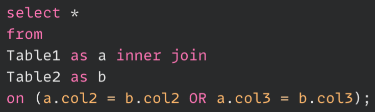
- Good
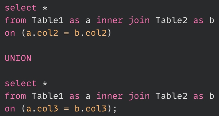
- Bad
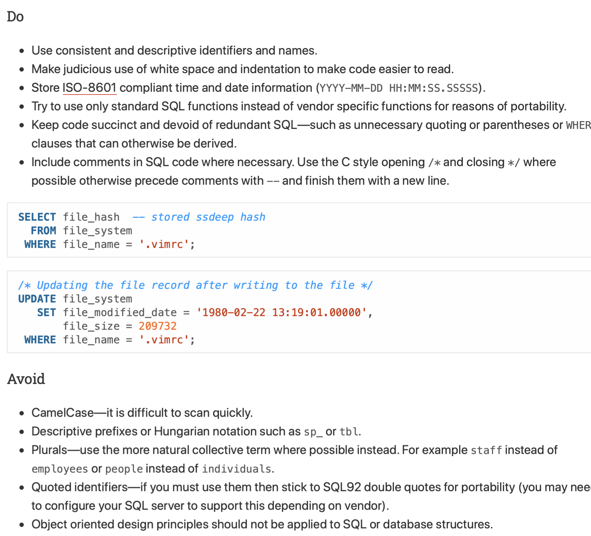
- Style Guide
Indexes
Misc
- An index may consist of up to 16 columns
- The first column of the index must always be present in the query’s filter, order , join or group operations to be used
Create Index on an existing table (postgres)
CREATE INDEX score_index ON grades(score, student);- “score_index” is the name of the index
- “grades” is the name of the table
- “score” and “student” are fields to be used as the indexes
Create Index that only uses a specific character length
/* mysql */ CREATE TABLE test (blob_col BLOB, INDEX(blob_col(10)));- index only uses the first 10 characters of the column value of a BLOB column type
Create index with multiple columns
/* mysql */
CREATE TABLE test (
    id        INT NOT NULL,
    last_name  CHAR(30) NOT NULL,
    first_name CHAR(30) NOT NULL,
    PRIMARY KEY (id),
    INDEX name (last_name,first_name)
)
Usage of multiple column index (** order of columns is important **)
SELECT * FROM test WHERE last_name='Jones';
SELECT * FROM test
  WHERE last_name='Jones' AND first_name='John';
SELECT * FROM test
  WHERE last_name='Jones'
  AND (first_name='John' OR first_name='Jon');
SELECT * FROM test
  WHERE last_name='Jones'
  AND first_name >='M' AND first_name < 'N';
Index is used when both columns are used as part of filtering criteria or when only the left-most column is used
if you have a three-column index on (col1, col2, col3), you have indexed search capabilities on (col1), (col1, col2), and (col1, col2, col3).
Invalid usage of multiple column index
SELECT * FROM test WHERE first_name='John'; SELECT * FROM test WHERE last_name='Jones' OR first_name='John';- The “name” index won’t be used in these queries since
- first_name is NOT the left-most column specified in the index
- OR is used instead of AND
- The “name” index won’t be used in these queries since
Create index with DESC, ASC
/* mysql */ CREATE TABLE t ( c1 INT, c2 INT, INDEX idx1 (c1 ASC, c2 ASC), INDEX idx2 (c1 ASC, c2 DESC), INDEX idx3 (c1 DESC, c2 ASC), INDEX idx4 (c1 DESC, c2 DESC) );- Used by
ORDER BY- See Docs to see what operations and index types support Descending Indexes
- Note: idx_a on column_p, column_q desc is not the same as an * Index idx_a on column_q desc, column p or, * Index idx_b on column_p desc, column q
- Used by
Usage of Descending Indexes
ORDER BY c1 ASC, c2 ASC -- optimizer can use idx1 ORDER BY c1 DESC, c2 DESC -- optimizer can use idx4 ORDER BY c1 ASC, c2 DESC -- optimizer can use idx2 ORDER BY c1 DESC, c2 ASC -- optimizer can use idx3- See previous example for definition of idx* names
- See Docs to see what operations and index types support Descending Indexes
Partitioning
- Misc
- Also see
- all of your queries to the partitioned table must contain the
partition_keyin theWHEREclause
Views
A smaller data object that contains the subset of data resulting from a specific query
If a table structure changes, the database can flag affected views for review.
Types
- Materialized Views
- Stores data and require refreshing
- Whereas a query happens after data is loaded, a materialized view is a precomputation (Basically, it’s a cached result)
- Can offer better performance for complex queries
- Standard Views
- Essentially saved queries that run each time you access the view. This means that when you query a standard view, you’re always seeing the current data in the underlying tables.
- Not separate storage
- Materialized Views
For Materialized Views and in postgres, you just need to replace
VIEWwithMATERIALIZED VIEWin the commandsCreate a View
Example: Create view as select (CVAS)
CREATE VIEW high_earner AS
SELECT p.id AS person_id, j.salary
FROM People p
JOIN Job j
ON p.job = j.title
WHERE j.salary >= 200000;
Query a view (same as a table):
SELECT * FROM high_earnerUpdate view
CREATE OR REPLACE VIEW high_earner AS SELECT p.id AS person_id, j.salary FROM People p JOIN Job j ON p.job = j.title WHERE j.salary >= 150000;- Expects the query output to retain the same number of columns, column names, and column data types. Thus, any modification that results in a change in the data structure will raise an error.
Change view name or a column name
ALTER VIEW foo RENAME TO bar;
ALTER VIEW foo RENAME COLUMN moose TO squirrel
Refresh Materialized View
Non-Concurrently
REFRESH MATERIALIZED VIEW view_name;- Might block users while view is being refreshed
- Best for cases in which a lot of rows are affected.
Concurrently
CREATE UNIQUE INDEX idx_view_name ON view_name (column1, column2); REFRESH MATERIALIZED VIEW CONCURRENTLY view_name;- Refreshes while not blocking other people using this view (i.e. concurrent access to view)
- Best for cases in which only a small number of rows are affected
- Requires index
List views
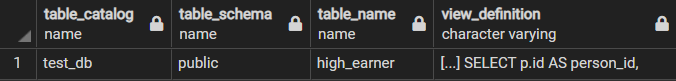
SELECT * FROM information_schema.views WHERE table_schema NOT IN ('pg_catalog', 'information_schema');- “table_name” has the names of the views
- “view_definition” shows the query stored in the view
- WHERE command is included to omit built-in views from PostgreSQL.
Delete view:
DROP VIEW high_earner;
Variables
- Misc
- Also see Business Queries >> Medians
- User-defined
DECLARE and SET
-- Declare your variables DECLARE @start date DECLARE @stop date -- SET the relevant values for each variable SET @start = '2021-06-01' SET @stop = GETDATE()- DECLARE sets the variable type (e.g. date)
- SET assigns a value
Or just use DECLARE
DECLARE @Iteration Integer = 0;Examples
Example: Exclude 3 months of data from the query
SELECT t1.[DATETIME], COUNT(*) AS vol FROM Medium.dbo.Earthquakes t1 WHERE t1.[DATETIME] BETWEEN @start AND DATEADD(MONTH, -3, @stop) GROUP BY t1.[DATETIME] ORDER BY t1.[DATETIME] DESC;- See above for the definitions of @start and @stop
Example: Apply a counter
-- Declare the variable (a SQL Command, the var name, the datatype)
DECLARE @counter INT;
-- Set the counter to 20
SET @counter = 20;
-- Print the initial value
SELECT @counter AS _COUNT;
-- Select and increment the counter by one
SELECT @counter = @counter + 1;
-- Print variable
SELECT @counter AS _COUNT;
-- Select and increment the counter by one
SELECT @counter += 1;
-- Print the variable
SELECT @counter AS _COUNT;
- System
- ROWCOUNT - returns the number of rows affected by the last previous statement
Example
BEGIN
    SELECT
        product_id,
        product_name
    FROM
        production.products
    WHERE
        list_price > 100000;
    IF @@ROWCOUNT = 0
        PRINT 'No product with price greater than 100000 found';
END
- ROWCOUNT - returns the number of rows affected by the last previous statement
Functions
“||” Concantenate strings. e.g ‘Post’ || ‘greSQL’ –> PostgreSQL
BEGIN…END- defines a compound statement or statement block. A compound statement consists of a set of SQL statements that execute together. A statement block is also known as a batch- A compound statement can have a local declaration for a variable, a cursor, a temporary table, or an exception
- Local declarations can be referenced by any statement in that compound statement, or in any compound statement nested within it.
- Local declarations are invisible to other procedures that are called from within a compound statement
- A compound statement can have a local declaration for a variable, a cursor, a temporary table, or an exception
COMMIT- a transaction control language that is used to permanently save the changes done in the transaction in tables/databases. The database cannot regain its previous state after its execution of commit.DATEADD- adds units of time to a variable or value- e.g.
DATEADD(month, -3, '2021-06-01')- subtracts 3 months from 2021-06-01
- e.g.
DATE_TRUNC- pulls a component of a date object.- e.g.
date_trunc('month', date_var) as month
- e.g.
DENSE_RANK- similar to theRANK, but it does not skip any numbers even if there is a tie between the rows.- Values are ranked by the column specified in ORDER BY expression of the window function
EXPLAIN- a means of running your query as a what-if to see what the planner thinks about it. It will show the process the system goes through to get to the data and return it.EXPLAIN SELECT s.id AS student_id, g.score FROM students AS s LEFT JOIN grades AS g ON s.id = g.student_id WHERE g.score > 90 ORDER BY g.score DESC; /* QUERY PLAN ---------- Sort (cost=80.34..81.88 rows=617 width=8) [...] Sort Key: g.score DESC [...] -> Hash Join (cost=16.98..51.74 rows=617 width=8) [...] Hash Cond: (g.student_id = s.id) [...] -> Seq Scan on grades g (cost=0.00..33.13 rows=617 width=8) [...] Filter: (score > 90) [...] -> Hash (cost=13.10..13.10 rows=310 width=4) [...] -> Seq Scan on students s (cost=0.00..13.20 rows=320 width=4) */- Sequentially scanning (“Seq Scan”) the grades and students tables because the tables aren’t indexed
- Any Seq Scan, parallel or not, is sub-optimal
EXPLAIN (BUFFERS)also shows how may data pages the database had to fetch using slow disk read operations (“read”), and how many of them were cached in memory (“shared hit”)- Also see
- Sequentially scanning (“Seq Scan”) the grades and students tables because the tables aren’t indexed
EXPLAIN ANALYZE- tells the planner to not only hypothesize on what it would do, but actually run the query and show the results.- Shows where indexes are being hit — or not hit as it may be. You can step through and re-optimize your basic and complex queries.
- Don’t use EXPLAIN ANALYZE on destructive operations like DELETE/UPDATE,EXPLAIN will suffice and it doesn’t run the query
- Don’t use EXPLAIN ANALYZE when resources are scarce like production monitoring, and when a query never finishes, EXPLAIN will suffice and it doesn’t run the query
- Also see Databases, Engineering >> Cost Optimizations
FILTER- Only the input rows for which the filter clause evaluates to true are fed to the aggregate function; other rows are discarded (postgres docs)- Especially useful when you want to perform multiple aggregations in your query.
- More readable than using CASE WHEN
- Also see
- Window Functions >>
- Calculate the number consecutive days spent in each country
- Three-day moving average of the temperature in each city
- Arrays >>
ARRAY_AGG
- Window Functions >>
- Example: Multiple Aggregations (source)
With FILTER
SELECT
    min(revenue) FILTER (WHERE make = ‘Ford’) min_ford,
    max(revenue) FILTER (WHERE make = ‘Ford’) max_ford,
    min(revenue) FILTER (WHERE make = ‘Renault’) min_renault,
    max(revenue) FILTER (WHERE make = ‘Renault’) max_renault
FROM
    car_sales;
With CASE WHEN
SELECT
    min(CASE WHEN make = ‘Ford’ THEN revenue ELSE null END) min_ford,
    max(CASE WHEN make = ‘Ford’ THEN revenue ELSE null END) max_ford,
    min(CASE WHEN make = ‘Renault’ THEN revenue ELSE null END) min_renault,
    max(CASE WHEN make = ‘Renault’ THEN revenue ELSE null END) max_renault
FROM
    car_sales;
GETDATE()- Gets the current dateGO- Not a sql function. Used by some interpreters as a reset.- i.e. any variables set before the GO statement will now not be recognized by the interpreter.
- Helps to separate code into different sections
ISDATE- boolean - checks that a variable is a date typeQUALIFY- clause filters the results of window functions.- useful when answering questions like fetching the most XXX value of each category
- QUALIFY does with window functions as what HAVING does with GROUP BY. As a result, in the order of execution, QUALIFY is evaluated after window functions.
- See Business Queries >> Get the latest order from each customer
UNION- It joins the outputs of two separate SELECT statements or tables. UNION keeps all rows in the first table/select statement or the second table/select statement. It also retains only one occurrence of duplicated rows if there are any.- i.e. It’s like if you
row_bindtwo dataframes and then only keep the unique rows.
- i.e. It’s like if you
UNNEST- BigQuery - takes an ARRAY and returns a table with a row for each element in the ARRAY (docs)- Google Analytics, Analysis >> Example 17
User Defined Functions (UDF)
Misc
- Available in SQL Server (Docs1, Docs2), Postgres (Docs), BigQuery (docs), etc.
- Keep a dictionary with the UDFs you’ve created and make sure to share it with any collaborators.
- Can be persistent or temporary
- Persistent UDFs can be used across multiple queries, while temporary UDFs only exist in the scope of a single query
Create
Example: temporary udf (BQ)
CREATE TEMP FUNCTION AddFourAndDivide(x INT64, y INT64) RETURNS FLOAT64 AS ( (x + 4) / y ); SELECT val, AddFourAndDivide(val, 2) FROM UNNEST([2,3,5,8]) AS val;Example: persistent udf (BQ)
CREATE FUNCTION mydataset.AddFourAndDivide(x INT64, y INT64)
RETURNS FLOAT64
AS (
  (x + 4) / y
);

SELECT
  val, mydataset.AddFourAndDivide(val, 2)
FROM
  UNNEST([2,3,5,8,12]) AS val;
Delete persistent udf:
DROP FUNCTION <udf_name>With Scalar subquery (BQ)
CREATE TEMP FUNCTION countUserByAge(userAge INT64)
AS (
  (SELECT COUNT(1) FROM users WHERE age = userAge)
);
SELECT
  countUserByAge(10) AS count_user_age_10,
  countUserByAge(20) AS count_user_age_20,
  countUserByAge(30) AS count_user_age_30;
Loops
- Misc
- posgres docs for loops
- WHILE
Example: Incrementally add to a counter variable
-- Declare the initial value
DECLARE @counter INT;
SET @counter = 20;
-- Print initial value
SELECT @counter AS _COUNT;
-- Create a loop
BEGIN;
-- Loop code starting point
WHILE @counter < 30
SELECT @counter = @counter + 1;
-- Loop finish
END;
-- Check the value of the variable
SELECT @counter AS _COUNT;
- Cursors (Docs)
Rather than executing a whole query at once, it is possible to set up a cursor that encapsulates the query, and then read the query result a few rows at a time.
- One reason for doing this is to avoid memory overrun when the result contains a large number of rows. (However, PL/pgSQL users do not normally need to worry about that, since FOR loops automatically use a cursor internally to avoid memory problems.)
- A more interesting usage is to return a reference to a cursor that a function has created, allowing the caller to read the rows. This provides an efficient way to return large row sets from functions.
Example (article (do not pay attention dynamic sql. it’s for embedding sql in C programs))
DECLARE cur_orders CURSOR FOR SELECT order_id, product_id, quantity FROM order_details WHERE product_id = 456; product_inventory INTEGER; BEGIN OPEN cur_orders; LOOP FETCH cur_orders INTO order_id, product_id, quantity; EXIT WHEN NOT FOUND; SELECT inventory INTO product_inventory FROM products WHERE product_id = 456; product_inventory := product_inventory - quantity; UPDATE products SET inventory = product_inventory WHERE product_id = 456; END LOOP; CLOSE cur_orders; -- do something after updating the inventory, such as logging the changes END;- A table called “products” that contains information about all products, including the product ID, product name, and current inventory. You can use a cursor to iterate through all orders that contain a specific product and update its inventory.
- A cursor called “cur_orders” that selects all order details that contain a specific product ID. We then define a variable called “product_inventory” to store the current inventory of the product.
- Inside the loop, we fetch each order ID, product ID, and quantity from the cursor, subtract the quantity from the current inventory and update the products table with the new inventory value.
- Finally, we close the cursor and do something after updating the inventory, such as logging the changes.
Window Functions
Unlike GROUP BY, keeps original columns after an aggregation
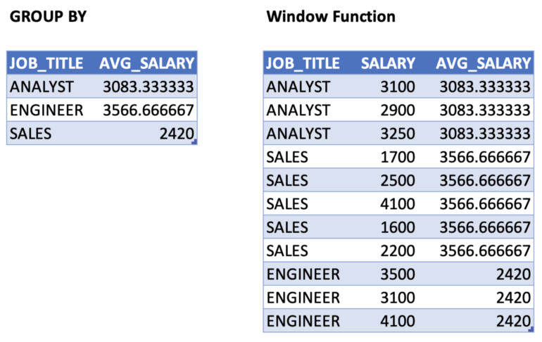
- Allows you to work with both aggregate and non-aggregate values all at once
- Better performance than using GROUP BY + JOIN to get the same result
- Allows you to work with both aggregate and non-aggregate values all at once
Despite the order of operations, if you really need to have a window function inside a WHERE clause or GROUP BY clause, you may get around this limitation by using a subquery or a WITH query
Example: Remove duplicate rows
WITH temporary_employees as
(SELECT
  employee_id,
  employee_name,
  department,
  ROW_NUMBER() OVER(PARTITION BY employee_name,
                                department,
                                employee_id) as row_count
FROM Dummy_employees)

SELECT *
FROM temporary_employees
WHERE row_count = 1
3 Types of Window Functions
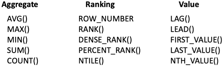
- LEAD() will give you the row AFTER the row you are finding a value for.
- LAG() will give you the row BEFORE the row you are finding a value for.
- FIRST_VALUE() returns the first value in an ordered, partitioned data output.
General Syntax
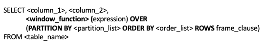
- window_function is the name of the window function we want to use (e.g. see above)
- expression is the name of the column that we want the window function operated on.
- May not be necessary depending on what window_function is used
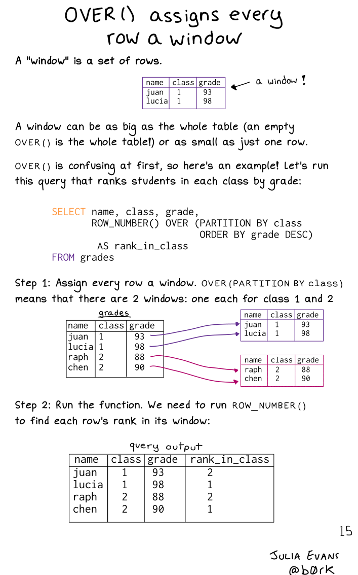
- OVER signifies that this is a window function
- expression is the name of the column that we want the window function operated on.
- PARTITION BY divides the rows into partitions so we can specify which rows to use to compute the window function
- partition_list is the name of the column(s) we want to partition by (i.e. group_by)
- ORDER BY is used so that we can order the rows within each partition. This is optional and does not have to be specified
- order_list is the name of the column(s) we want to order by
- ROWS (optional; typically not used) used to subset the rows within each partition.
- frame_clause defines how much to offset from our current row
- Syntax: ROWS BETWEEN <starting_row> AND <ending_row>
- Options for starting and ending row
- UNBOUNDED PRECEDING — all rows before the current row in the partition, i.e. the first row of the partition
- [some #] PRECEDING — # of rows before the current row
- CURRENT ROW — the current row
- [some #] FOLLOWING — # of rows after the current row
- UNBOUNDED FOLLOWING — all rows after the current row in the partition, i.e. the last row of the partition
- Examples
- ROWS BETWEEN 3 PRECEDING AND CURRENT ROW — this means look back the previous 3 rows up to the current row.
- ROWS BETWEEN UNBOUNDED PRECEDING AND 1 FOLLOWING — this means look from the first row of the partition to 1 row after the current row
- ROWS BETWEEN 5 PRECEDING AND 1 PRECEDING — this means look back the previous 5 rows up to 1 row before the current row
- ROWS BETWEEN UNBOUNDED PRECEDING AND UNBOUNDED FOLLOWING — this means look from the first row of the partition to the last row of the partition
- Options for starting and ending row
- window_function is the name of the window function we want to use (e.g. see above)
Example: Average Salary by Job Title
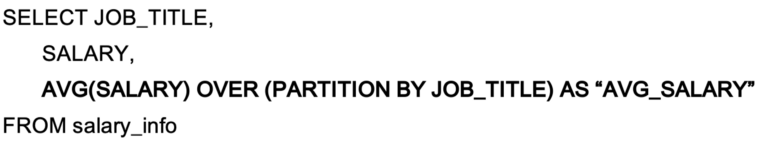
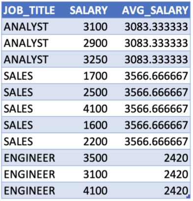
Tables for Examples
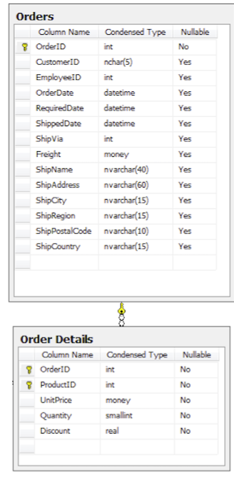
Example: Average Unit Price for each CustomerId
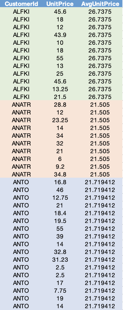
SELECT CustomerId, UnitPrice, AVG(UnitPrice) OVER (PARTITION BY CustomerId) AS “AvgUnitPrice” FROM [Order] INNER JOIN OrderDetail ON [Order].Id = OrderDetail.OrderIdExample: Average Unit Price for each group of CustomerId AND EmployeeId
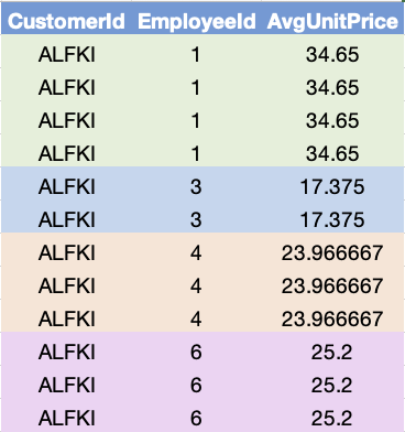
SELECT CustomerId, EmployeeId, AVG(UnitPrice) OVER (PARTITION BY CustomerId, EmployeeId) AS “AvgUnitPrice” FROM [Order] INNER JOIN OrderDetail ON [Order].Id = OrderDetail.OrderIdExample: Create a new column that ranks Unit Price in descending order for each CustomerId
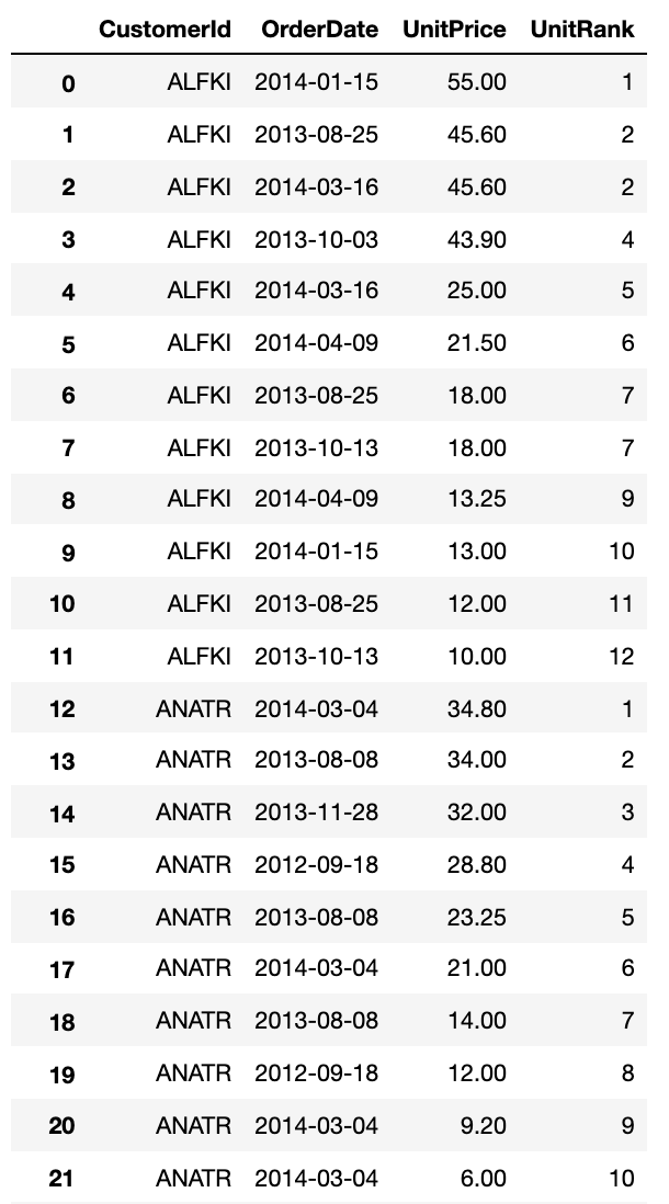
SELECT CustomerId, OrderDate, UnitPrice, ROW_NUMBER() OVER (PARTITION BY CustomerId ORDER BY UnitPrice DESC) AS “UnitRank” FROM [Order] INNER JOIN OrderDetail ON [Order].Id = OrderDetail.OrderId- Substituting RANK in place of ROW_NUMBER should produce the same results
- Note that ranks are skipped (e.g. rank 3 for ALFKI) when there are rows with the same rank
- If you don’t want ranks skipped, use DENSE_RANK for the window function
Example: Create a new column that provides the previous order date’s Quantity for each ProductId
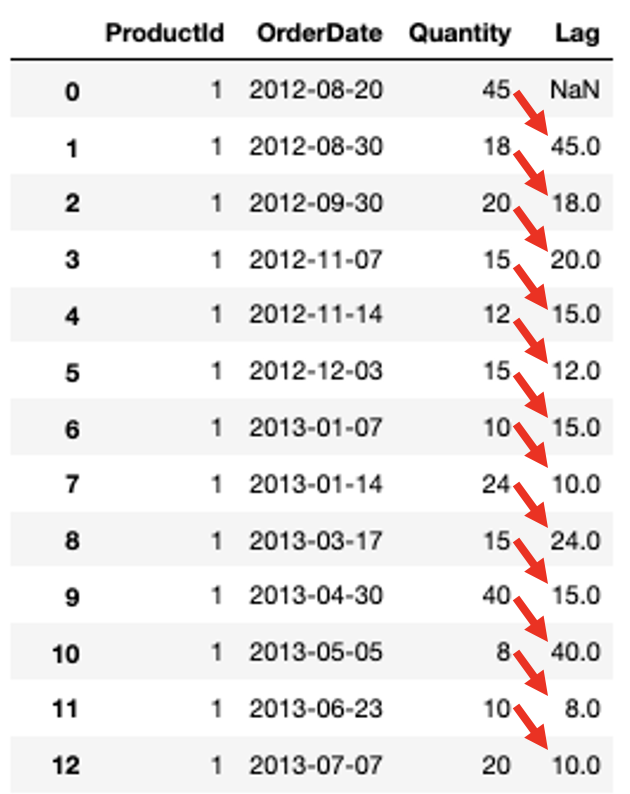
SELECT ProductId, OrderDate, Quantity, LAG(Quantity) OVER (PARTITION BY ProductId ORDER BY OrderDate) AS "LAG" FROM [Order] INNER JOIN OrderDetail ON [Order].Id = OrderDetail.OrderId- Use LEAD for the following quantity
Example: Create a new column that provides the very first Quantity ever ordered for each ProductId
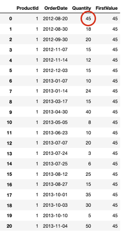
SELECT ProductId, OrderDate, Quantity, FIRST_VALUE(Quantity) OVER (PARTITION BY ProductId ORDER BY OrderDate) AS "FirstValue" FROM [Order] INNER JOIN OrderDetail ON [Order].Id = OrderDetail.OrderIdExample: Calculate a cumulative moving average UnitPrice for each CustomerId
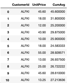
SELECT CustomerId, UnitPrice, AVG(UnitPrice) OVER (PARTITION BY CustomerId ORDER BY CustomerId ROWS BETWEEN UNBOUNDED PRECEDING AND CURRENT ROW) AS “CumAvg” FROM [Order] INNER JOIN OrderDetail ON [Order].Id = OrderDetail.OrderIdExample: Rank customers for each department by amount spent
SELECT customer_name, customer_id, amount_spent, department_id, RANK(amount_spent) OVER(ORDER BY amount_spent DESC PARTITION BY department_id) AS spend_rank FROM employeesExample: Find the model and year of car that been on lot the longest
SELECT
FIRST_VALUE(name) OVER(PARTITION BY model, year ORDER BY date_at_lot ASC) AS oldest_car_name
model,
year
FROM cars
Running Totals/Averages (Cumulative Sums)
Uses
SUMas the window function- Just replace SUM with AVG to get running averages
Example
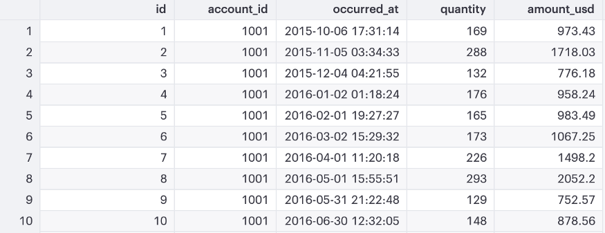
- Generate a new dataset grouped by month, instead of timestamp. (CTE)
- Only include three fields: account_id, occurred_month and total_amount_usd
- Only computed for the following accounts: 1041 , 1051, 1061, 10141.
- Compute a running total ordered by occurred_month, without collapsing the rows in the result set.
- Display 2 columns: occurred_month and cum_amnt_usd_by_month
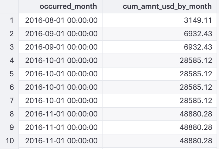
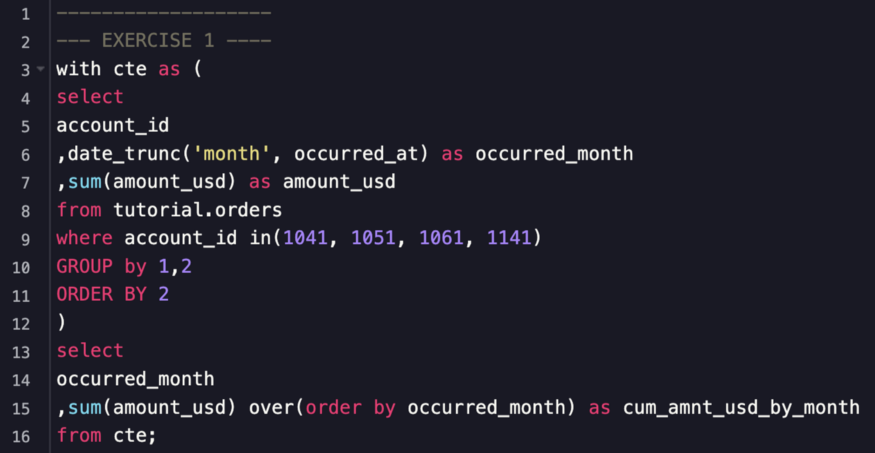
- Display 2 columns: occurred_month and cum_amnt_usd_by_month
- Because no partition was specified, the running total is applied on the full dataset and ordered by (ascending) occurred_month
- Generate a new dataset grouped by month, instead of timestamp. (CTE)
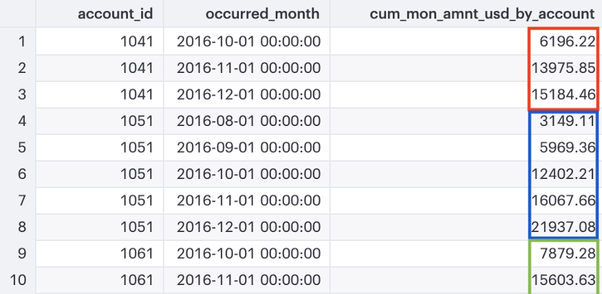
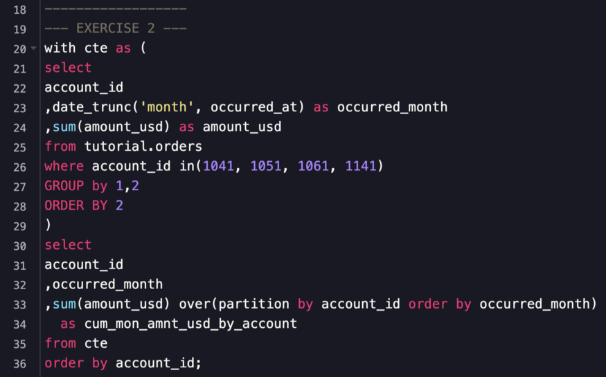
Example running total by grouping variable
- Using previous CTE
- Compute a running total by account_id, ordered by occurred_month, and account_id (i.e. a separate running total for each account_id.)
- Display 3 columns: account_id, occurred_month, and cum_mon_amnt_usd_by_account
- Display 3 columns: account_id, occurred_month, and cum_mon_amnt_usd_by_account
- Compute a running total by account_id, ordered by occurred_month, and account_id (i.e. a separate running total for each account_id.)
- Same as previous example except a partition column (account_id) is added
- Using previous CTE
Example Running total over various window lengths
- Using previous CTE
- Compute a 3 months rolling running total using a window that includes the current month.
- Compute a 7 months rolling running total using a window where the current month is always the middle month.
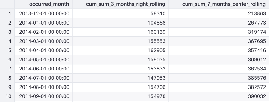
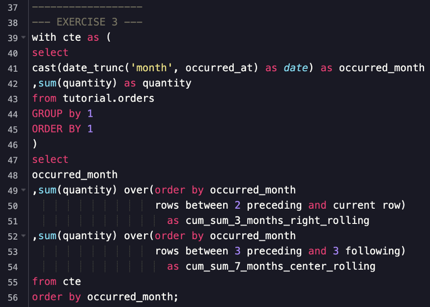
- First case uses 2 PRECEDING rows and the CURRENT_ROW
- Second case uses 3 PRECEDING rows and 3 FOLLOWING rows and the CURRENT_ROW
- Using previous CTE
Example: Calculate the number consecutive days spent in each country (sqlite)
with ordered as ( select created, country, lag(country) over (order by created desc) as previous_country from raw ), grouped as ( select country, created, count(*) filter ( where previous_country is null or previous_country != country ) over ( order by created desc rows between unbounded preceding and current row ) as grp from ordered ) select country, date(min(created)) as start, date(max(created)) as end, cast( julianday(date(max(created))) - julianday(date(min(created))) as integer ) as days from grouped group by country, grp order by start desc;-
- Goes over the code and thought process step-by-step with shows original data and results during intermediate steps
-
- Evidently only sqlite and postgres support filter. Someone in the thread suggest an alternate method.
Output:
country         start         end           days
United Kingdom  2023-06-08  2023-06-08  0
United States   2019-09-02  2023-05-11  1347
France          2019-08-25  2019-08-31  6
Madagascar      2019-07-31  2019-08-07  7
France          2019-07-25  2019-07-25  0
United States   2019-05-04  2019-06-30  57
United Kingdom  2018-08-29  2018-09-10  12
United States   2018-08-05  2018-08-10  5
-
Example: Three-day moving average of the temperature in each city (postgres, source)
SELECT city, day, temperature,
    MAX(temperature) FILTER (WHERE temperature > 70)
    OVER (
      PARTITION BY city
      ORDER BY day ASC
      ROWS BETWEEN 2 PRECEDING AND CURRENT ROW) max_3day
FROM city_data
ORDER BY city, day;
Common Table Expressions (CTE)
The result set of a query which exists temporarily and for use only within the context of a larger query. Much like a derived table, the result of a CTE is not stored and exists only for the duration of the query.
Also see
- Window Functions >> Running Totals >> Examples
- Google, Google Analytics, Analysis >> Examples 12-15, 18, 19
Use Cases
- Needing to reference a derived table multiple times in a single query
- An alternative to creating a view in the database
- Performing the same calculation multiple times over across multiple query components
Improves readability and usually no performance difference
- Prior to PostgreSQL 12, https://hakibenita.com/be-careful-with-cte-in-postgre-sql , something with the caching mechanism created a bottleneck. Currently, version 13 is the latest, so hopefully not a common problem anymore.
Steps
- Initiate a CTE using “WITH”
- Provide a name for the result soon-to-be defined query
- After assigning a name, follow with “AS”
- Specify column names (optional step)
- Define the query to produce the desired result set
- If multiple CTEs are required, initiate each subsequent expression with a comma and repeat steps 2-4.
- Reference the above-defined CTE(s) in a subsequent query
Syntax
WITH
expression_name_1 AS
(CTE query definition 1)
[, expression_name_X AS
  (CTE query definition X)
, etc ]
SELECT expression_A, expression_B, ...
FROM expression_name_1
Example
Comparison with a “derived” query
“What is the average monthly cost per campaign for the company’s marketing efforts?”
Using CTE workflow
-- define CTE:
WITH Cost_by_Month AS
(SELECT campaign_id AS campaign,
      TO_CHAR(created_date, 'YYYY-MM') AS month,
      SUM(cost) AS monthly_cost
FROM marketing
WHERE created_date BETWEEN NOW() - INTERVAL '3 MONTH' AND NOW()
GROUP BY 1, 2
ORDER BY 1, 2)

-- use CTE in subsequent query:
SELECT campaign, avg(monthly_cost) as "Avg Monthly Cost"
FROM Cost_by_Month
GROUP BY campaign
ORDER BY campaign
Used derived query
-- Derived
SELECT campaign, avg(monthly_cost) as "Avg Monthly Cost"
FROM
    -- this is where the derived query is used
    (SELECT campaign_id AS campaign,
      TO_CHAR(created_date, 'YYYY-MM') AS month,
      SUM(cost) AS monthly_cost
    FROM marketing
    WHERE created_date BETWEEN NOW() - INTERVAL '3 MONTH' AND NOW()
    GROUP BY 1, 2
    ORDER BY 1, 2) as Cost_By_Month
GROUP BY campaign
ORDER BY campaign
Example
- Count the number of interactions of new users
- Steps
- Get new users
- Count interactions
- Get interactions of new users
WITH new_users AS (
    SELECT id
    FROM users
    WHERE created >= '2021-01-01'
),
count_interactions AS (
    SELECT id,
        COUNT(*) n_interactions
    FROM interactions
    GROUP BY id
),
interactions_by_new_users AS (
    SELECT id,
        n_interactions
    FROM new_users
        LEFT JOIN count_interactions USING (id)
)

SELECT *
FROM interactions_by_new_users
Example
Find the average top Math test score for students in California
Steps
- Get a subset of students (California)
- Get a subset of test scores (Math)
- Join them together to get all Math test scores from California students
- Get the top score per student
- Take the overall average
Derived Query (i.e. w/o CTE)
SELECT AVG(score)
FROM
  (SELECT students.id, MAX(test_results.score) as score
  FROM students
  JOIN schools ON (
    students.school_id = schools.id AND schools.state = 'CA'
  )
  JOIN test_results ON (
    students.id = test_results.student_id
    AND test_results.subject = 'math'
  )
  GROUP BY students.id) as tmp
Using CTE
WITH
  student_subset as (
    SELECT students.id
    FROM students
    JOIN schools ON (
      students.school_id = schools.id AND schools.state = 'CA'
    )
  ),
  score_subset as (
    SELECT student_id, score
    FROM test_results
    WHERE subject = 'math'
  ),
  student_scores as (
    SELECT student_subset.id, score_subset.score
    FROM student_subset
    JOIN score_subset ON (
        student_subset.id = score_subset.student_id
    )
  ),
  top_score_per_student as (
    SELECT id, MAX(score) as score
    FROM student_scores
    GROUP BY id
  )

SELECT AVG(score)
FROM top_score_per_student
Strings
Concatenate
Also see Processing Expressions >> NULLs
“||”
SELECT 'PostgreSQL' || ' ' || 'Databases' AS result; result -------------- PostgreSQL DatabasesCONCATSELECT CONCAT('PostgreSQL', ' ', 'Databases') AS result; result -------------- PostgreSQL DatabasesWith NULL values
SELECT CONCAT('Harry', NULL, 'Peter'); -------------- HarryPeter- “||” won’t work with NULLs
Columns
SELECT first_name, last_name, CONCAT(first_name,' ' , last_name) "Full Name" FROM candidates;- New column, “Full Name”, is created with concatenated columns
Splitting (BQ)
SELECT *, CASE WHEN ARRAY_LENGTH(SPLIT(page_location, '/')) >= 5 AND CONTAINS_SUBSTR(ARRAY_REVERSE(SPLIT(page_location, '/'))[SAFE_OFFSET(0)], '+') AND (LOWER(SPLIT(page_location, '/')[SAFE_OFFSET(4)]) IN ('accessories','apparel','brands','campus+collection','drinkware', 'electronics','google+redesign', 'lifestyle','nest','new+2015+logo','notebooks+journals', 'office','shop+by+brand','small+goods','stationery','wearables' ) OR LOWER(SPLIT(page_location, '/')[SAFE_OFFSET(3)]) IN ('accessories','apparel','brands','campus+collection','drinkware', 'electronics','google+redesign', 'lifestyle','nest','new+2015+logo','notebooks+journals', 'office','shop+by+brand','small+goods','stationery','wearables' ) ) THEN 'PDP' WHEN NOT(CONTAINS_SUBSTR(ARRAY_REVERSE(SPLIT(page_location, '/'))[SAFE_OFFSET(0)], '+')) AND (LOWER(SPLIT(page_location, '/')[SAFE_OFFSET(4)]) IN ('accessories','apparel','brands','campus+collection','drinkware', 'electronics','google+redesign', 'lifestyle','nest','new+2015+logo','notebooks+journals', 'office','shop+by+brand','small+goods','stationery','wearables' ) OR LOWER(SPLIT(page_location, '/')[SAFE_OFFSET(3)]) IN ('accessories','apparel','brands','campus+collection','drinkware', 'electronics','google+redesign', 'lifestyle','nest','new+2015+logo','notebooks+journals', 'office','shop+by+brand','small+goods','stationery','wearables' ) ) THEN 'PLP' ELSE page_title END AS page_title_adjusted FROM unnested_events- From article, gist
- Query is creating a new categorical column, “page_title_adjusted,” that is “PDP” when a substring in “page_location” is one of a set of words, and “PLP” when it’s not, and the value of page_title otherwise.
- SPLIT splits the string by separator, ‘/’
- CONTAINS_SUBSTR is looking for substring with a “+”
- [SAFE_OFFSET(3)] pulls the 4th substring (think this indexes by 0?)
- After it’s been reversed via ARRAY_REVERSE (?)
- ELSE says use the value for page_title when length of the substrings after splitting page_location is 5 or less
- “unnested_events” is a CTE
Arrays
Misc
- PostGres
- Indexing Arrays starts at 1, not at 0
- PostGres
Create Array (BQ)
SELECT ARRAY
  (SELECT 1 UNION ALL
  SELECT 2 UNION ALL
  SELECT 3) AS new_array;
+-----------+
| new_array |
+-----------+
| [1, 2, 3] |
+-----------+

SELECT
  ARRAY
    (SELECT AS STRUCT 1, 2, 3
    UNION ALL SELECT AS STRUCT 4, 5, 6) AS new_array;
+------------------------+
| new_array              |
+------------------------+
| [{1, 2, 3}, {4, 5, 6}] |
+------------------------+

SELECT ARRAY
  (SELECT AS STRUCT [1, 2, 3] UNION ALL
  SELECT AS STRUCT [4, 5, 6]) AS new_array;
+----------------------------+
| new_array                  |
+----------------------------+
| [{[1, 2, 3]}, {[4, 5, 6]}] |
+----------------------------+
Create a table with Arrays (Postgres)
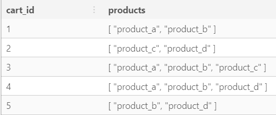
CREATE TEMP TABLE shopping_cart ( cart_id serial PRIMARY KEY, products text ARRAY ); INSERT INTO shopping_cart(products) VALUES (ARRAY['product_a', 'product_b']), (ARRAY['product_c', 'product_d']), (ARRAY['product_a', 'product_b', 'product_c']), (ARRAY['product_a', 'product_b', 'product_d']), (ARRAY['product_b', 'product_d']); -- alt syntax w/o ARRAY INSERT INTO shopping_cart(products) VALUES ('{"product_a", "product_d"}');- Also see Basics >> Add Data >> Example: chatGPT
Subset an array (postgres)
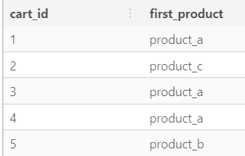
SELECT
  cart_id,
  products[1] AS first_product -- indexing starts at 1
FROM
  shopping_cart;
Slice an array (postgres)
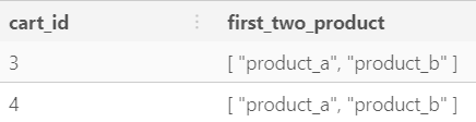
SELECT
  cart_id,
  products [1:2] AS first_two_products
FROM
  shopping_cart
WHERE
  CARDINALITY(products) > 2;
Unnest an array (postgres)
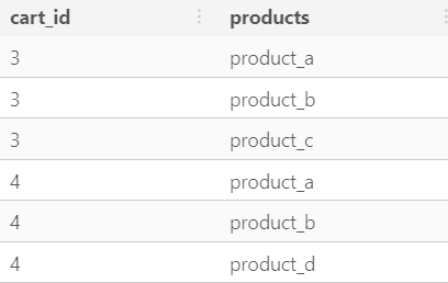
SELECT cart_id, UNNEST(products) AS products FROM shopping_cart WHERE cart_id IN (3, 4);- Useful if you want to perform a join
Filter according to items in arrays (postgres)
SELECT cart_id, products FROM shopping_cart WHERE 'product_c' = ANY (products);- Only rows with arrays that have “product_c” will be returned
Change array values using
UPDATE,SET-- update arrays UPDATE shopping_cart SET products = ARRAY['product_a','product_b','product_e'] WHERE cart_id = 1; UPDATE shopping_cart SET products[1] = 'product_f' WHERE cart_id = 2; SELECT * FROM shopping_cart ORDER BY cart_id;First update: all arrays where cart_id == 1 are set to [‘product_a’,‘product_b’,‘product_e’]
Second update: all array first values where cart_id == 2 are set to ‘product_f’
Insert array values
ARRAY_APPEND- puts value at the end of the arrayUPDATE shopping_cart SET products = ARRAY_APPEND(products, 'product_x') WHERE cart_id = 1;- arrays in product column where cart_id == 1 get “product_x” appended to the end of their arrays
ARRAY_PREPEND- puts value at the beginning of the arrayUPDATE shopping_cart SET products = ARRAY_PREPEND('product_x', products) WHERE cart_id = 2;- arrays in product column where cart_id == 2 get “product_x” prepended to the beginning of their arrays
ARRAY_REMOVE- remove array itemUPDATE shopping_cart SET products = array_remove(products, 'product_e') WHERE cart_id = 1;- arrays in product column where cart_id == 1 get “product_e” removed from their arrays
ARRAY_CONCAT(BQ),ARRAY_CAT(postgres) - ConcantenateSELECT ARRAY_CONCAT([1, 2], [3, 4], [5, 6]) as count_to_six; +--------------------------------------------------+ | count_to_six | +--------------------------------------------------+ | [1, 2, 3, 4, 5, 6] | +--------------------------------------------------+ -- postgres SELECT cart_id, ARRAY_CAT(products, ARRAY['promo_product_1', 'promo_product_2']) FROM shopping_cart ORDER BY cart_id;ARRAY_TO_STRING- Coerce to string (BQ)WITH items AS (SELECT ['coffee', 'tea', 'milk' ] as list UNION ALL SELECT ['cake', 'pie', NULL] as list) SELECT ARRAY_TO_STRING(list, '--') AS text FROM items; +--------------------------------+ | text | +--------------------------------+ | coffee--tea--milk | | cake--pie | +--------------------------------+ WITH items AS (SELECT ['coffee', 'tea', 'milk' ] as list UNION ALL SELECT ['cake', 'pie', NULL] as list) SELECT ARRAY_TO_STRING(list, '--', 'MISSING') AS text FROM items; +--------------------------------+ | text | +--------------------------------+ | coffee--tea--milk | | cake--pie--MISSING | +--------------------------------+ARRAY_AGG- gather values of a group by variable into an array (doc)Makes the output more readable
Example: Get categories for each brand
-- without array_agg select brand, category from order_item group by brand, category order by brand, category ; Results: | brand | category | | ------ | ---------- | | Arket | jacket | | COS | shirts | | COS | trousers | | COS | vest | | Levi's | jacket | | Levi's | jeans | -- with array_agg select brand, array_agg(distinct category) as all_categories from order_item group by brand order by brand ; Results: | brand | all_categories | | ------ | ---------------------------- | | Arket | ['jacket'] | | COS | ['shirts','trousers','vest'] | | Levi's | ['jacket','jeans'] | | Uniqlo | ['shirts','t-shirts','vest'] |Example: With FILTER in a CTE (postgres?, source)
1-- without group by with product_users as ( select array_agg(user_id) filter (where doc_storage = true) as doc_storage_users, array_agg(user_id) filter (where photo_storage = true) as photo_storage_users from Sales ) 2-- with group by with product_users as ( select user_category, array_agg(user_id) filter (where doc_storage = true) as doc_storage_users, array_agg(user_id) filter (where photo_storage = true) as photo_storage_users from Sales group by user_category )- 1
-
I think the author wanted an array output, but to also use
FILTER.FILTERcan only be used with aggregate functions. This shows thatARRAY_AGGdoesn’t necessarily needGROUP BYfunction - 2
- Customers are aggregated by the storage they bought and their user category
ARRAY_SIZE- function takes an array or a variant as input and returns the number of items within the array/variant (doc)Example: How many categories does each brand have?
select
  brand,
  array_agg(distinct category) as all_categories,
  array_size(all_categories) as no_of_cat
from order_item
group by brand
order by brand
;
Results:
| brand  | all_categories              | no_of_cat |
| ------ | ---------------------------  | --------- |
| Arket  | ['jacket']                  | 1        |
| COS    | ['shirts','trousers','vest'] | 3        |
| Levi's | ['jacket','jeans']          | 2        |
| Uniqlo | ['shirts','t-shirts','vest'] | 3        |

-- postgres using CARDINALITY to get array_size
SELECT
  cart_id,
  CARDINALITY(products) AS num_products
FROM
  shopping_cart;
ARRAY_CONTAINSchecks if a variant is included in an array and returns a boolean value. (doc)Variant is just a specific category
Need to cast the item you’d like to check as a variant first
Syntax:
ARRAY_CONTAINS(variant, array)Example: What brands have jackets?
select brand, array_agg(distinct category) as all_categories, array_size(all_categories) as no_of_cat, array_contains('jacket'::variant,all_categories) as has_jacket from order_item group by brand order by brand ; Results: | brand | all_categories | no_of_cat | has_jacket | | ------ | --------------------------- | --------- | ---------- | | Arket | ['jacket'] | 1 | true | | COS | ['shirts','trousers','vest'] | 3 | false | | Levi's | ['jacket','jeans'] | 2 | true | | Uniqlo | ['shirts','t-shirts','vest'] | 3 | false | -- postgres contains_operator, @> SELECT cart_id, products FROM shopping_cart WHERE products @> ARRAY['product_a', 'product_b'];- “@>” example returns all rows with arrays containing product_a and product_b
Business Queries
Total Sales, Customers, Sales per Customer per Region
SELECT region, SUM(sales) as total_sales, COUNT(DISTINCT customer_id) as customer_count, SUM(sales) / COUNT(DISTINCT customer_id) as sales_per_customer FROM read_csv('sales_data*.csv') WHERE sale_date >= '2024-01-01' GROUP BY region ORDER BY total_sales DESC- DuckDB SQL allows you to read directly from a csv
Simple Moving Average (SMA)
Example: 7-day SMA including today
SELECT
  Date, Conversions,
  AVG(Conversions) OVER (ORDER BY Date ROWS BETWEEN 6 PRECEDING AND
  CURRENT ROW) as SMA
FROM daily_sales
Example: 3-day SMA not including today
select date, sales, avg(sales) over (order by date rows between 3 preceding and current row - 1) as moving_avg from table_daily_salesExample: Rank product categories by shipping cost for each shipping address
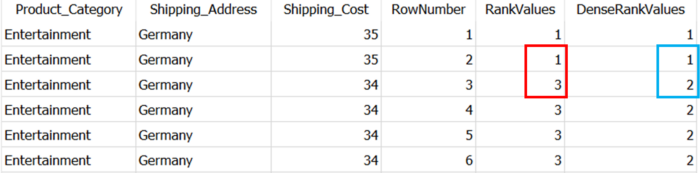
SELECT Product_Category, Shipping_Address, Shipping_Cost, ROW_NUMBER() OVER (PARTITION BY Product_Category, Shipping_Address ORDER BY Shipping_Cost DESC) as RowNumber, RANK() OVER (PARTITION BY Product_Category, Shipping_Address ORDER BY Shipping_Cost DESC) as RankValues, DENSE_RANK() OVER (PARTITION BY Product_Category, Shipping_Address ORDER BY Shipping_Cost DESC) as DenseRankValues FROM Dummy_Sales_Data_v1 WHERE Product_Category IS NOT NULL AND Shipping_Address IN ('Germany','India') AND Status IN ('Delivered')RANK()retrieves ranked rows based on the condition ofORDER BYclause. As you can see there is a tie between 1st two rows i.e. first two rows have same value in Shipping_Cost column (which is mentioned in ORDER BY clause).DENSE_RANKis similar to theRANK, but it does not skip any numbers even if there is a tie between the rows. This you can see in Blue box in the above picture.- Rank resets to 1 when “Shipping_Address” changes location
Example: Total order quantity for each month
SELECT strftime('%m', OrderDate) as Month, SUM(Quantity) as Total_Quantity from Dummy_Sales_Data_v1 GROUP BY strftime('%m', OrderDate)strftimeextracts the month (%m) from the datetime column, “OrderDate”
Example: Monthly and yearly number of orders and average shipping costs
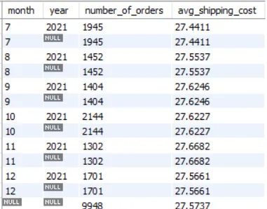
SELECT EXTRACT(MONTH FROM order_date) AS month
    , EXTRACT(YEAR FROM order_date) AS year
    , COUNT(orderid) AS number_of_orders
    , AVG(shipping_cost) AS avg_shipping_cost
FROM alldata.salesdata
GROUP BY EXTRACT(MONTH FROM order_date)
       , EXTRACT(YEAR FROM order_date) WITH ROLLUP;
The last row in the above result, where you see
NULLin both month and year columns indicates that it shows results for all months in all years i.e. it gives you a total number of orders and average shipping cost in the year 2021.WITH ROLLUPat the end of theGROUP BYclause says performCOUNTandAVGover the whole year. If there were more than one year, I’m not sure if it would compute the values for each year or for the whole time period though.
Example: Daily counts of open jobs
- The issue is that there aren’t rows for transactions that remain in a type of holding status
- e.g. Job Postings website has date columns for the date the job posting was created, the date the job posting went live on the website, and the date the job posting was taken down (action based timestamps), but no dates for the status between “went live” and “taken down”.
-- create a calendar column SELECT parse_datetime('2020–01–01 08:00:00', 'yyyy-MM-dd H:m:s') + (interval '1' day * d) as cal_date from FROM ( SELECT ROW_NUMBER() OVER () -1 as d FROM (SELECT 0 as n UNION SELECT 1) p0, (SELECT 0 as n UNION SELECT 1) p1, (SELECT 0 as n UNION SELECT 1) p2, (SELECT 0 as n UNION SELECT 1) p3, (SELECT 0 as n UNION SELECT 1) p4, (SELECT 0 as n UNION SELECT 1) p5, (SELECT 0 as n UNION SELECT 1) p6, (SELECT 0 as n UNION SELECT 1) p7, (SELECT 0 as n UNION SELECT 1) p8, (SELECT 0 as n UNION SELECT 1) p9, (SELECT 0 as n UNION SELECT 1) p10 ) -- left-join your table to the calendar column Select c.cal_date, count(distinct opp_id) as "historical_prospects" From calendar c Left Join opportunities o on o.stage_entered ≤ c.cal_date and (o.stage_exited is null or o.stage_exited > c.cal_date)- Calendar column should probably be a CTE
- Notes from Using SQL to calculate trends based on historical status
- Some flavours of SQL have a generate_series function, which will create this calendar column for you
- For one particular month, then create an indicator column with “if posting_publish_date ≤ 2022–01–01 and (posting_closed_date is null or posting_closed_date > 2022–01–31) then True” and then filter for True and count.
- The issue is that there aren’t rows for transactions that remain in a type of holding status
Example: Get the latest order from each customer
-- Using QUALIFY
select
    date,
    customer_id,
    order_id,
    price
from customer_order_table
qualify row_number() over (partition by customer_id order by date desc) = 1
;

-- CTE w/window function
with order_order as
(
select
    date,
    customer_id,
    order_id,
    price,
    row_number() over (partition by customer_id order by date desc)
    as order_of_orders
from customer_order_table
)

select
    *
from order_order
where order_of_orders = 1
;
Results:
| date      | customer_id | order_id | price |
|------------|-------------|----------|-------|
| 2022-01-03 | 002        | 212      | 350  |
| 2022-01-06 | 005        | 982      | 300  |
| 2022-01-07 | 001        | 109      | 120  |
Medians
Notes from How to Calculate Medians with Grouping in MySQL
Variables:
pid: unique id variable
category: A or B
price: random value between 1 and 6
Example: Overall median price
SELECT AVG(sub.price) AS median
FROM (
    SELECT @row_index := @row_index + 1 AS row_index, p.price
    FROM products.prices p, (SELECT @row_index := -1) r
    WHERE p.category = 'A'
    ORDER BY p.price
) AS sub
WHERE sub.row_index IN (FLOOR(@row_index / 2), CEIL(@row_index / 2))
;

median|
------+
   3.0|
@row_index is a SQL variable that is initiated in the
FROMstatement and updated for each row in theSELECTstatement.The column whose median will be calculated (the price column in this example) should be sorted. It doesn’t matter if it’s sorted in ascending or descending order.
According to the definition of median, the median is the value of the middle element (total count is odd) or the average value of the two middle elements (total count is even). In this example, category A has 5 rows and thus the median is the value of the third row after sorting. The values of both
FLOOR(@row_index / 2)andCEIL(@row_index / 2)are 2 which is the third row. On the other hand, for category B which has 6 rows, the median is the average value of the third and fourth rows.
Example: Median price for each product
SELECT
    sub2.category,
    CASE WHEN MOD(sub2.total, 2) = 1 THEN sub2.mid_prices
         WHEN MOD(sub2.total, 2) = 0 THEN (SUBSTRING_INDEX(sub2.mid_prices, ',', 1) + SUBSTRING_INDEX(sub2.mid_prices, ',', -1)) / 2
    END AS median
FROM
    (
        SELECT
            sub1.category,
            sub1.total,
            CASE WHEN MOD(sub1.total, 2) = 1 THEN SUBSTRING_INDEX(SUBSTRING_INDEX(sub1.prices, ',', CEIL(sub1.total/2)), ',', '-1')
                 WHEN MOD(sub1.total, 2) = 0 THEN SUBSTRING_INDEX(SUBSTRING_INDEX(sub1.prices, ',', sub1.total/2 + 1), ',', '-2')
            END AS mid_prices
        FROM
            (
                SELECT
                    p.category,
                    GROUP_CONCAT(p.price ORDER BY p.price) AS prices,
                    COUNT(*) AS total
                FROM products.prices p
                GROUP BY p.category
            ) sub1
    ) sub2
;

category|median|
--------+------+
A       |3     |
B       |3.5   |
Breaking down the subqueries
Sort prices per category
SELECT category, GROUP_CONCAT(price ORDER BY p.price) AS prices, COUNT(*) AS total FROM products.prices p GROUP BY p.category ; category|prices |total| --------+-----------+-----+ A |1,2,3,4,5 | 5| B |1,2,3,4,5,6| 6|- If your table has a lot of data, GROUP_CONCAT would not contain all the data. In this case, you increase the limit for GROUP_CONCAT by:
SET GROUP_CONCAT_MAX_LEN = 100000;
- If your table has a lot of data, GROUP_CONCAT would not contain all the data. In this case, you increase the limit for GROUP_CONCAT by:
Get middle prices according to whether the total count is an odd or even number
SELECT
    sub1.category,
    sub1.total,
    CASE WHEN MOD(sub1.total, 2) = 1 THEN SUBSTRING_INDEX(SUBSTRING_INDEX(sub1.prices, ',', CEIL(sub1.total/2)), ',', '-1')
         WHEN MOD(sub1.total, 2) = 0 THEN SUBSTRING_INDEX(SUBSTRING_INDEX(sub1.prices, ',', sub1.total/2 + 1), ',', '-2')
    END AS mid_prices
FROM
    (
        SELECT
            p.category,
            GROUP_CONCAT(p.price ORDER BY p.price) AS prices,
            COUNT(*) AS total
        FROM products.prices p
        GROUP BY p.category
    ) sub1
;

category|total|mid_prices|
--------+-----+----------+
A       |    5|3         |
B       |    6|3,4       |
We use the
MODfunction (modulo) to check if the total count is an odd or even number.The
SUBSTRING_INDEXfunction is used twice to extract the middle elements.
Example: Overall median of price and quantity
SELECT
    CASE WHEN MOD(sub2.total, 2) = 1 THEN sub2.mid_prices
         WHEN MOD(sub2.total, 2) = 0 THEN (SUBSTRING_INDEX(sub2.mid_prices, ',', 1) + SUBSTRING_INDEX(sub2.mid_prices, ',', -1)) / 2
    END AS median_of_price,
    CASE WHEN MOD(sub2.total, 2) = 1 THEN sub2.mid_quantities
         WHEN MOD(sub2.total, 2) = 0 THEN (SUBSTRING_INDEX(sub2.mid_quantities, ',', 1) + SUBSTRING_INDEX(sub2.mid_prices, ',', -1)) / 2
    END AS median_of_quantity
FROM
    (
        SELECT
            sub1.total,
            CASE WHEN MOD(sub1.total, 2) = 1 THEN SUBSTRING_INDEX(SUBSTRING_INDEX(sub1.prices, ',', CEIL(sub1.total/2)), ',', '-1')
                 WHEN MOD(sub1.total, 2) = 0 THEN SUBSTRING_INDEX(SUBSTRING_INDEX(sub1.prices, ',', sub1.total/2 + 1), ',', '-2')
            END AS mid_prices,
            CASE WHEN MOD(sub1.total, 2) = 1 THEN SUBSTRING_INDEX(SUBSTRING_INDEX(sub1.quantities, ',', CEIL(sub1.total/2)), ',', '-1')
                 WHEN MOD(sub1.total, 2) = 0 THEN SUBSTRING_INDEX(SUBSTRING_INDEX(sub1.quantities, ',', sub1.total/2 + 1), ',', '-2')
            END AS mid_quantities
        FROM
            (
                SELECT
                    COUNT(*) AS total,
                    GROUP_CONCAT(o.price ORDER BY o.price) AS prices,
                    GROUP_CONCAT(o.quantity ORDER BY o.quantity) AS quantities
                FROM products.orders o
            ) sub1
    ) sub2
;


median_of_price|median_of_quantity|
---------------+------------------+
3              |30                |
Similar to previous example
Variables: order_id, price, quantity
Transactions
Misc
- Also see
- Terms >> Transaction
- Database, Warehouses >> Database Triggers - Shows how to efficiently transfer data from a transactional database to a warehouse/relational database by setting up event triggers and staging tables.
- When the transaction is successful, COMMIT is applied. When the transaction is aborted, incorrect execution, system failure ROLLBACK occurs.
- Also see
Only used with INSERT, UPDATE and DELETE
BEGIN TRANSACTION: It indicates the start point of an explicit or local transaction.- Represents a point ast which the data referenced by a connection is logically and physically consistent.
- If errors are encountered, all data modifications made after the BEGIN TRANSACTION can be rolled back to return the data to this known state of consistency
- Syntax:
BEGIN TRANSACTION transaction_name ;
SET TRANSACTION: Places a name on a transaction.- Syntax:
SET TRANSACTION [ READ WRITE | READ ONLY ];
- Syntax:
COMMIT: used to permanently save the changes done in the transaction in tables/databases. The database cannot regain its previous state after its execution of commit.If everything is in order with all statements within a single transaction, all changes are recorded together in the database is called committed. The COMMIT command saves all the transactions to the database since the last COMMIT or ROLLBACK command
Example: Delete records
DELETE FROM Student WHERE AGE = 20; COMMIT;- Deletes those records from the table which have age = 20 and then commits the changes in the database.
ROLLBACK: used to undo the transactions that have not been saved in the database. The command is only been used to undo changes since the last commit- If any error occurs with any of the SQL grouped statements, all changes need to be aborted. The process of reversing changes is called rollback. This command can only be used to undo transactions since the last COMMIT or ROLLBACK command was issued.
- Syntax:
ROLLBACK;
SAVEPOINT: creates points within the groups of transactions in which to ROLLBACK.Syntax:
SAVEPOINT <savepoint_name>;A savepoint is a point in a transaction in which you can roll the transaction back to a certain point without rolling back the entire transaction.
Remove a savepoint:
RELEASE SAVEPOINT <savepoint_name>Example: Rollback a deletion
SAVEPOINT SP1;
//Savepoint created.
DELETE FROM Student WHERE AGE = 20;
//deleted
SAVEPOINT SP2;
//Savepoint created.
ROLLBACK TO SP1;
//Rollback completed.
Processing Expressions
Use multiple conditions in a WHERE expression
select * from XXX_table where 1=1 (if condition A) and clause 1 (if condition B) and clause 2 (if condition C) and clause 3 ;- The “1=1” prevents errors that would occur when the first condition doesn’t apply to any rows.
- Can also use “true”
- The “1=1” prevents errors that would occur when the first condition doesn’t apply to any rows.
Select unique rows without using DISTINCT
Using UNION
SELECT employee_id, employee_name, department FROM Dummy_employees UNION SELECT employee_id, employee_name, department FROM Dummy_employees- there must be same number and order of columns in both the SELECT statements
Using INTERSECT
SELECT employee_id, employee_name, department FROM Dummy_employees INTERSECT SELECT employee_id, employee_name, department FROM Dummy_employees- There must be same number and order of columns in both the SELECT statements
Using ROW_NUMBER
WITH temporary_employees as (
  SELECT
    employee_id,
    employee_name,
    department,
    ROW_NUMBER() OVER(PARTITION BY employee_name,
                                  department,
                                  employee_id) as row_count
  FROM Dummy_employees
)

SELECT *
FROM temporary_employees
WHERE row_count = 1
Using GROUP BY
SELECT employee_id, employee_name, department FROM Dummy_employees GROUP BY employee_id, employee_name, department- Just need to group by all the columns. Useful to use in conjunction with aggregate functions.
CASE WHEN
SELECT OrderID,
      OrderDate,
      Sales_Manager,
      Quantity,
      CASE WHEN Quantity > 51 THEN 'High'
            WHEN Quantity < 51 THEN 'Low'
            ELSE 'Medium'
      END AS OrderVolume
FROM Dummy_Sales_Data_v1
END ASspecifies the name of the new column, “OrderVolume”ELSEspecifies the value when none of the conditions are met- If you did not mention ELSE clause and no condition is satisfied, the query will return NULL for that specific record
Pivot Wider
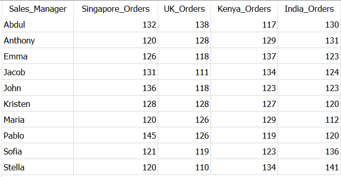
SELECT Sales_Manager, COUNT(CASE WHEN Shipping_Address = 'Singapore' THEN OrderID END) AS Singapore_Orders, COUNT(CASE WHEN Shipping_Address = 'UK' THEN OrderID END) AS UK_Orders, COUNT(CASE WHEN Shipping_Address = 'Kenya' THEN OrderID END) AS Kenya_Orders, COUNT(CASE WHEN Shipping_Address = 'India' THEN OrderID END) AS India_Orders FROM Dummy_Sales_Data_v1 GROUP BY Sales_Manager- Depending on your use-case you can also use different aggregation such as SUM, AVG, MAX, MIN with CASE statement.
NULLs
Division and NULLS
Any division with NULL values with have a result of NULL.
isNullallows to get a different resulting valueSELECT IsNull(<column>, 0) / 45- All NULL values in the column will replaced with 0s during the division operation.
COALESCESubstitute a default value in place of NULLs
SELECT COALESCE(column_name, 'Default Value') AS processed_column FROM table_name; SELECT COALESCE(order_date, current_date) AS processed_date FROM orders; SELECT product ||' - '|| COALESCE(subcategory, category, family, 'no product description ') AS product_and_subcategory FROM stock- 3rd Expression: If there is a NULL in subcategory, then it looks in category, then into family, and finally if all those fields have NULLs, it uses “no product description” as the value.
Concantenating Strings where NULLs are present
SELECT COALESCE(first_name, '') || ' ' || COALESCE(last_name, '') AS full_name FROM employees;- NULLs are replaced with an empty string so transformation doesn’t break
Performing calculations involving numeric columns where there are NULLs
SELECT COALESCE(quantity, 0) * COALESCE(unit_price, 0) AS total_cost FROM products; SELECT product, quantity_available, minimum_to_have, COALESCE(minimum_to_have, quantity_available * 0.5) AS threshold FROM stock- NULLs are substituted with 0s so the calcuation doesn’t break
As part of a join in case keys have missing values
SELECT *
FROM employees e
LEFT JOIN departments d ON COALESCE(e.department_id, 0) = COALESCE(d.id, 0);
With Aggregate Functions
SELECT department_id, COALESCE(SUM(salary), 0) AS total_salary
FROM employees
GROUP BY department_id;
Make hierarchical subtotals output more readable
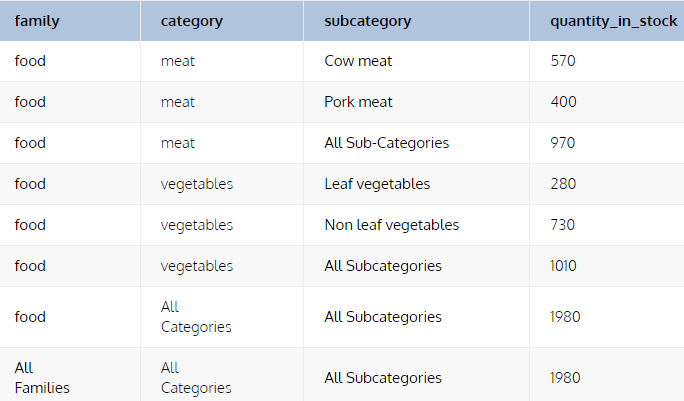
SELECT COALESCE(family,'All Families') AS family, COALESCE(category,'All Categories') AS category, COALESCE(subcategory,'All Subcategories') AS subcategory, SUM(quantity_available) as quantity_in_stock FROM stock GROUP BY ROLLUP(family, category, subcategory) ORDER BY family, category, subcategoryROLLUPclause assumes a hierarchy among the columnsfamily,category, andsubcategory. Thus, it generates all the grouping sets that make sense considering the hierarchy:GROUP BY family,GROUP BY family, categoryandGROUP BY family, category, subcategory.- This is the reason why
ROLLUPis often used to generate subtotals and grand totals for reports.
- This is the reason why
Without
COALESCE, the text in the unused columns for the subtotals would be NULLs.
Duplicated Rows
Uses
QUALIFYas a window function to filter out duplicates/* removes duplicate rows at the order_id level */ SELECT * FROM orders QUALIFY row_number() over (partition by order_id order by created_at) = 1More verbose example of what’s happening
WITH temporary_employees as
(SELECT
  employee_id,
  employee_name,
  department,
  ROW_NUMBER() OVER(PARTITION BY employee_name,
                                department,
                                employee_id) as row_count
FROM Dummy_employees)

SELECT *
FROM temporary_employees
WHERE row_count = 1
Use a hash column as id column, then test for duplicates, remove them or investigate them (BigQuery)
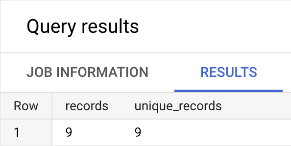
WITH inbound_zoo_elephants AS ( SELECT * FROM flowfunctions.examples.zoo_elephants ), add_row_hash AS ( SELECT *, TO_HEX(MD5(TO_JSON_STRING(inbound_zoo_elephants))) AS hex_row_hash FROM inbound_zoo_elephants ) SELECT COUNT(*) AS records, COUNT(DISTINCT hex_row_hash) AS unique_records FROM add_row_hash- No duplicate records found, since “records” = 9 and “unique_records” = 9
- if records > unique_records, duplicates exist
- Can select distinct hex_row_hash if you want to remove duplicates
- Can count hex_row_hash then filter where hex_row_hash > 1 to find which rows are duplicates
- Notes from link
- Description
- flowfunctions is the project name
- examples is a directory (?)
- zoo_elephants is the dataset
- Steps
- TO_JSON_STRING - creates column with json string for each row
- MD5 hashes that string
- TO_HEX makes it alpha-numeric and gets rid of the symbols in the hash
- Easier to deal with in BigQuery
- Assume this is still unique (?)
- Note: By adding “true” value,
TO_JSON_STRING(inbound_zoo_elephants, true), TO_JSON_STRING adds line breaks to the json string for easier readability. - Hashing function options
- MD5 - shortest one (16 characters), fine for this use case
- cryptographically broken, returns 16 characters and suffices for our use-case. Other options are
- FARM_FINGERPRINT - returns a signed integer of variable length
- SHA1, SHA256 and SHA512, which return 20, 32 and 64 bytes respectively and are more secure for cryptographic use cases.
- MD5 - shortest one (16 characters), fine for this use case
- No duplicate records found, since “records” = 9 and “unique_records” = 9
Nested Data
- Recursive CTE
Recursive CTEs are used primarily when you want to query hierarchical data or graphs. This could be a company’s organizational structure, a family tree, a restaurant menu, or various routes between cities
Also see
- What Is a Recursive CTE in SQL?
- Tutorial, 3 examples, and links to other articles
- What Is a Recursive CTE in SQL?
Syntax
WITH RECURSIVE cte_name AS ( cte_query_definition (the anchor member) UNION ALL cte_query_definition (the recursive member) ) SELECT * FROM cte_name;Example: : postgres
WITH RECURSIVE category_tree(id, name, parent_id, depth, path) AS ( SELECT id, name, parent_id, 1, ARRAY[id] FROM categories WHERE parent_id IS NULL UNION ALL SELECT categories.id, categories.name, categories.parent_id, category_tree.depth + 1, path || categories.id FROM categories JOIN category_tree ON categories.parent_id = category_tree.id ) SELECT id, name, parent_id, depth, path FROM category_tree;- CTE (
WITH) +RECURSIVEsays it’s a recursive query. UNION ALLcombines the results of both statements.- Example is defined by 2 Select statements
- Anchor Member: First SELECT statement selects the root nodes of the category tree (nodes with no parent)
- Root node is indicated by “parent_id” = NULL
- Recursive member: Second SELECT statement selects the child nodes recursively
- Anchor Member: First SELECT statement selects the root nodes of the category tree (nodes with no parent)
- Also see Arrays for further examples of the use of
UNION ALL
- Example is defined by 2 Select statements
- The “depth” column is used to keep track of the depth of each category node in the tree.
- “1” in the first statement
- “category_tree.depth + 1” in the second statement
- With every recursion, the CTE will add 1 to the previous depth level, and it will do that until it reaches the end of the hierarchy
- The “path” column is an array that stores the path from the root to the current node.
- “ARRAY[id]” in the first statement
- “path || categories.id” in the second statement
- “||” concatenates “path” and “id” columns (See Strings)
- CTE (
Binning
CASE WHEN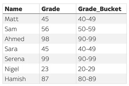
SELECT Name, Grade, CASE WHEN Grade < 10 THEN '0-9' WHEN Grade BETWEEN 10 and 19 THEN '10-19' WHEN Grade BETWEEN 20 and 29 THEN '20-29' WHEN Grade BETWEEN 30 and 39 THEN '30-39' WHEN Grade BETWEEN 40 and 49 THEN '40-49' WHEN Grade BETWEEN 50 and 59 THEN '50-59' WHEN Grade BETWEEN 60 and 69 THEN '60-69' WHEN Grade BETWEEN 70 and 79 THEN '70-79' WHEN Grade BETWEEN 80 and 89 THEN '80-89' WHEN Grade BETWEEN 90 and 99 THEN '90-99' END AS Grade_Bucket FROM studentsBETWEENis inclusive of the end points- Flexible for any size of bin you need
FLOORSELECT Name, Grade, FLOOR(Grade / 10) * 10 AS Grade_Bucket FROM students- Can easily scale up the number of bins without having to increase the lines of code
- Only useful for evenly spaced bins
LEFT JOIN on preformatted tableCREATE OR REPLACE TABLE bins ( Lower_Bound INT64, Upper_Bound INT64, Grade_Bucket STRING ); INSERT bins (Lower_Bound, Upper_Bound, Grade_Bucket) VALUES (0, 9, '0-9') (10, 19, '10-19') (20, 29, '20-29') (30, 39, '30-39') (40, 49, '40-49') (50, 59, '50-59') (60, 69, '60-69') (70, 79, '70-79') (80, 89, '80-89') (90, 99, '90-99'); SELECT A.Name, A.Grade, B.Grade_Bucket FROM students AS A LEFT JOIN bins AS B ON A.Grade BETWEEN B.Lower_Bound AND B.Upper_Bound- “bins” table acts a template that funnels the values from your table into the correct bins
Time Series
All the records between two dates
SELECT * FROM alldata.salesdata WHERE 1=1 AND order_date BETWEEN '2021-08-01' AND '2021-08-31'; /* without BETWEEN */ SELECT * FROM alldata.salesdata WHERE 1=1 AND order_date >= '2021-08-01' AND order_date <= '2021-08-31';- Without BETWEEN is not optimized and therefore, not recommended
Extract components from date-time columns
/* MySQL */ SELECT EXTRACT(YEAR FROM order_date) AS year , EXTRACT(MONTH FROM order_date) AS month , EXTRACT(QUARTER FROM order_date) AS quarter , EXTRACT(WEEK FROM order_date) AS week_of_year , EXTRACT(DAY FROM order_date) AS day_of_month , EXTRACT(HOUR FROM order_date) AS hour_of_day , EXTRACT(MINUTE FROM order_date) AS minute_of_hour , EXTRACT(SECOND FROM order_date) AS second_of_minute , order_date FROM alldata.salesdata; /* SQLte */ SELECT strftime('%m', OrderDate) as Monthstrftimecodes
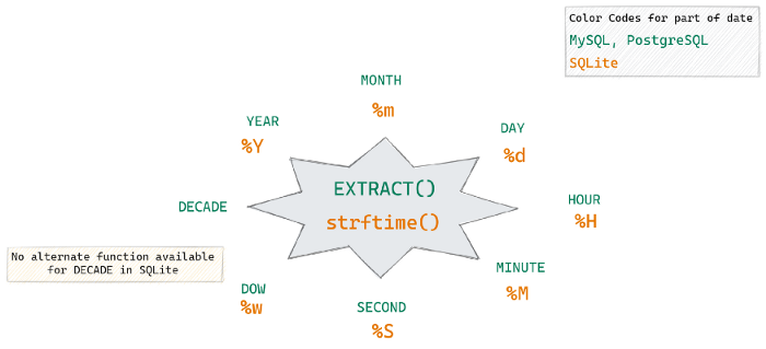
Preprocess Time Series with 4 Lags (article)
WITH top_customers as ( --- select the customter ids you want to track ), transactions as ( SELECT cust_id, dt, date_trunc('hour', cast(event_time as timestamp)) as event_hour, count(*) as transactions FROM ourTable WHERE dt between cast(date_add('day', -7, current_date) as varchar) and cast(current_date as varchar) GROUP BY 1,2,3 Order By event_hour asc ) SELECT transactions.cust_id, transactions.event_hour, day_of_week(transactions.event_hour) day_of_week, hour(transactions.event_hour) hour_of_day, transactions.transactions as transactions, LAG(transactions,1) OVER (PARTITION BY transactions.cust_id ORDER BY event_hour) AS lag1, LAG(transactions,2) OVER (PARTITION BY transactions.cust_id ORDER BY event_hour) AS lag2, LAG(transactions,3) OVER (PARTITION BY transactions.cust_id ORDER BY event_hour) AS lag3, LAG(transactions,4) OVER (PARTITION BY transactions.cust_id ORDER BY event_hour) AS lag4 FROM transactions join top_customers on transactions.cust_id = top_customers.cust_id /* output */ "cust_id", "event_hour", "day_of_week", "hour_of_day", "transactions", "lag1", "lag2", "lag3", "lag4" "Customer-123","2023-01-14 00:00:00.000","6","0","4093",,,,,, "Customer-123","2023-01-14 01:00:00.000","6","1","4628","4093",,,,, "Customer-123","2023-01-14 02:00:00.000","6","2","5138","4628","4093",,,, "Customer-123","2023-01-14 03:00:00.000","6","3","5412","5138","4628","4093",,, "Customer-123","2023-01-14 04:00:00.000","6","4","5645","5412","5138","4628","4093", "Customer-123","2023-01-14 05:00:00.000","6","5","5676","5645","5412","5138","4628", "Customer-123","2023-01-14 06:00:00.000","6","6","6045","5676","5645","5412","5138", "Customer-123","2023-01-14 07:00:00.000","6","7","6558","6045","5676","5645","5412",- Dataset contains number of transactions made per customer per hour.
- 2 WITH clauses: the first just extracts a list of customers we are interested in. Here you can add any condition that is supposed to filter in or out specific customers (perhaps you want to filter new customers or only include customers with sufficient traffic). The second WITH clause simply creates the first data set — Dataset A, which pulls a week of data for these customers and selects the customer id, date, hour, and number of transactions.
- Finally, the last and most important SELECT clause generates Dataset B, by using SQL lag() function on each row in order to capture the number of transactions in each of the hours that preceded the hour in the row.
Tools
- ChatSQL - Convert plain text to MySQL query by ChatGPT
- databow (docs, intro) - A open source command-line tool for querying any database that has an ADBC (Arrow Database Connectivity) driver. Built in Rust, databow gives you one fast, modern interface to the SQL systems across your entire data stack
Includes:
Transactional databases: PostgreSQL, MySQL, MariaDB, SQLite, Oracle Database, Microsoft SQL Server, CockroachDB, YugabyteDB, TiDB
Analytical databases: DuckDB, ClickHouse, Snowflake, BigQuery, Databricks, Amazon Redshift, Teradata
Lakehouse engines: Trino, Dremio, StarRocks, Apache Doris
Time-series databases: InfluxDB, TimescaleDB, GreptimeDB
- ggsql - Allows pure SQL users to create ggplot2 style visualizations via a sql query. Based on grammar of graphics. More reproducible than using a gui-based tool
- Works inside of positron, vs code, jupyter, quarto
- Easier for LLMs to use since they’re very good at sql
- Embedding a small executable in other tools is much easier than bundling R/Python (or requiring them to be installed)
- e.g. lighter to use in remote production environment than installing R/Python
- A smaller scope makes it easier to sandbox and prevent malicious code execution (either deliberately or in error)
- SQLFluff - A rust-based, dialect-flexible, configurable SQL linter. Designed with ELT applications in mind and will auto-fix most linting errors.
- Also works with Jinja templating and dbt. SQLFluff
- {sqlfluffr} - An R interface to the ‘Python’ ‘sqlfluff’ ‘SQL’ linter and formatter via the ‘reticulate’ package.
- Includes special handling for ‘glue’ ‘SQL’ syntax with curly-brace placeholders
- {sqlglot} - no dependency Python SQL parser, transpiler, optimizer, and engine
Format SQL or translate between nearly twenty different SQL dialects.
- It doesn’t just transpile active SQL code, too. Moves comments from one dialect to another.
The parser itself can be customized
Can also help you analyze queries, traverse parsed expression trees, and incrementally (and, programmatically) build SQL queries.
support for optimizing SQL queries, and performing semantic diffs.
Can be used to unit test queries through mocks based on Python dictionaries.
Example: : translate duckdb to hive
import sqlglot
sqlglot.transpile(
  "SELECT EPOCH_MS(1618088028295)",
  read = "duckdb",
  write = "hive"
)[0]
---
'SELECT FROM_UNIXTIME(1618088028295 / 1000)'
- sqlit - A user friendly Terminal UI (TUI) for SQL databases
- Supports all major databases: SQL Server, PostgreSQL, MySQL, SQLite, MariaDB, FirebirdSQL, Oracle, DuckDB, CockroachDB, ClickHouse, Snowflake, Supabase, CloudFlare D1, Turso, Athena, BigQuery, RedShift, IBM Db2, SAP HANA, Teradata, Trino, Presto and Apache Flight SQL.
- Automatically finds running database containers
- SQL Studio - SQL Database Explorer [SQLite, libSQL, PostgreSQL, MySQL/MariaDB, DuckDB]