Training

• Packages
  • {autokeras} - Leverages Neural Architecture Search (NAS) techniques behind the scenes. It uses a trial-and-error approach powered by Keras Tuner under the hood to test different configurations. Once a good candidate is found, it trains it to convergence and evaluates.
  • {keras-tuner} - Focused on hyperparameter optimization. You define the search space (e.g., number of layers, number of units, learning rates), and it uses optimization algorithms (random search, Bayesian optimization, Hyperband) to find the best configuration.
• Resources
  • Automating Deep Learning: A Gentle Introduction to AutoKeras and Keras Tuner
    • Basic intro to {autokeras} and {keras-tuner}
• Use early stopping and set the number of iterations arbitrarily high. This removes the chance of terminating learning too early.
• Symplectic Optimization
  • FromWhat to Do When Your Credit Risk Model Works Today, but Breaks Six Months Later (Code) (See IEEE DSA2025 for paper)
  • Claims to forestall model drift (AUC) for months later than gradient descent optimizers (e.g. ADAM)
  • Use as alternative to gradient descent optimizers when
    • Ranking matters more than classification accuracy
    • Distribution shift is gradual and predictable (economic cycles, not black swans)
    • Temporal stability is critical (financial risk, medical prognosis over time)
    • Retraining is expensive (regulatory validation, approval overhead)
    • You can afford 2–3x training time for production stability
    • You have <10K features (works well up to ~10K dimensions)
  • Don’t use when:

    • Distribution shift is abrupt/unpredictable (market crashes, regime changes)

    • You need interpretability for compliance (this doesn’t help with explainability)

    • You’re in ultra-high dimensions (>10K features, cost becomes prohibitive)

    • Real-time training constraints (2–3x slower than Adam)

• Strategies
  
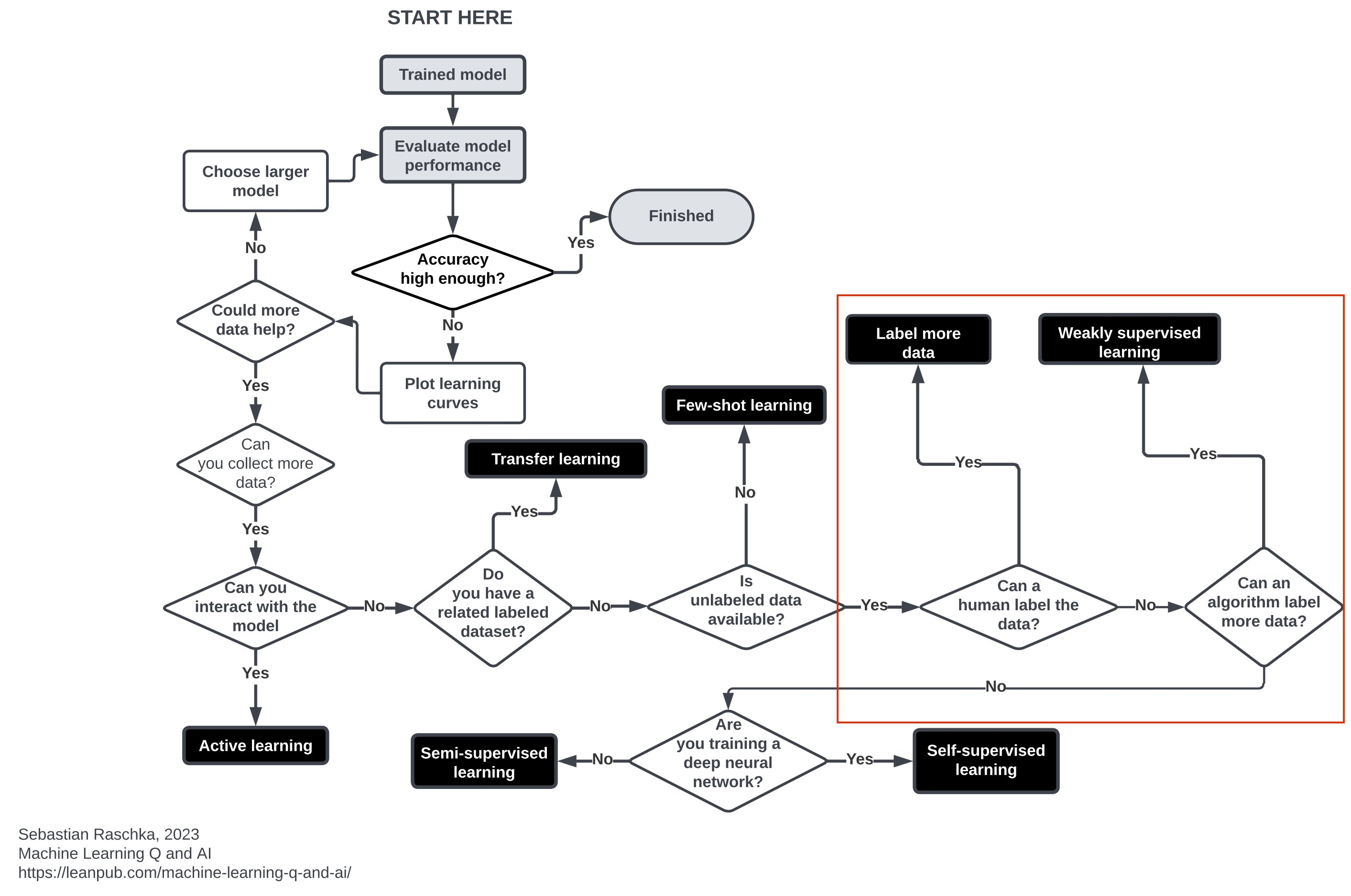
  • Includes Active Learning, Transfer Learning, Few-Shot Learning, Weakly-Supervised Learning, Self-Supervised Learning, Semi-Supervised Learning
• Common Variations of Gradient Descent
  • Batch Gradient Descent: Use the entire training dataset to compute the gradient of the loss function. This is the most robust but not computationally feasible for large datasets.
  • Stochastic Gradient Descent: Use a single data point to compute the gradient of the loss function. This method is the quickest but the estimate can be noisy and the convergence path slow.
  • Mini-Batch Gradient Descent: Use a subset of the training dataset to compute the gradient of the loss function. The size of the batches varies and depends on the size of the dataset. This is the best of both worlds of both batch and stochastic gradient descent.
    • Use the largest batch sizes possible that can fit inside your computer’s GPU RAM as they parallelize the computation
• High-Frequency Checkpoints
  • Notes from I Measured Neural Network Training Every 5 Steps for 10,000 Iterations
  • {ndtracker}
  • e.g. training a DNN with 10,000 steps, you traditionally set up chack points every 100 or 200 or even 500 steps. Setting up high frequency checkpoints would mean setting them up every 5 or so steps.
  • Provide information about:
    • Whether early training mistakes can be recovered from (they often can’t)
    • Why some architectures work and others fail
    • When interpretability analysis should happen (spoiler: way earlier than we thought)
    • How to design better training approaches
  • Use Cases:
    • Intervention experiments that map causal dependencies
      • Disrupt training during specific windows and measure which downstream capabilities are lost. If corrupting data during steps 2,000-5,000 permanently damages texture recognition but the same corruption at step 6,000 has no effect, you’ve found when texture features crystallize and what they depend on. This works identically for object recognition in vision models, syntactic structure in language models, or state discrimination in RL agents.
    • For production deployment, continuous dimensionality monitoring catches representational problems during training when you can still fix them.
      • If layers stop expanding, you have architectural bottlenecks. If expansion becomes erratic, you have instability. If early layers saturate while late layers fail to expand, you have information flow problems. Standard loss curves won’t show these issues until it’s too late—dimensionality tracking surfaces them immediately.
    • Measure expansion dynamics during the first 5-10% of training across candidate architectures. Select for clean phase transitions and structured bottom-up development.
      • These networks aren’t just more performant—they’re fundamentally more interpretable because features form in clear sequential layers rather than tangled simultaneity.
  • Ansuini et al. discovered the effective representational dimensionality increases during training (Confirmed by Yang et al, 2024), i.e. the learning space expands (model is more complex) while the network learns.
  • Phases:
    • Phase 1: Collapse (steps 0-300) The network restructures from random initialization. Dimensionality drops sharply as the loss landscape is reshaped around the task. This isn’t learning yet, it’s preparation for learning.
    • Phase 2: Expansion (steps 300-5,000) Dimensionality climbs steadily. This is capacity expansion. The network is building representational structures. Simple features that enable complex features that enable higher-order features.
    • Phase 3: Stabilization (steps 5,000-8,000) Growth plateaus. Architectural constraints bind. The network refines what it has rather than building new capacity.
  • Two thirds of all transitions happen in the first 2,000 steps — just 25% of total training time. If we want to understand what features form and when, we need to look during steps 0-2,000, not at convergence.
  • In real deployment scenarios, we can track representational dimensionality in real-time, detect when expansion phases occur, and run interpretability analyses at each transition point. This tells us precisely when our network is building new representational structures—and when it’s finished
• GPU methods
  
• Data Storage
  • Data samples are iteratively loaded from a storage location and fed into the DL model
    • The speed of each training step and, by extension, the overall time to model convergence, is directly impacted by the speed at which the data samples can be loaded from storage
  • Which metrics are important depends on the application
    • Time to first sample might be important in a video application
    • Average sequential read time and Total processing time would be important for DL models
  • Factors
    • Data Location: The location of the data and its distance from the training machine can impact the latency of the data loading.
    • Bandwidth: The bandwidth on the channel of communication between the storage location and the training machine will determine the maximum speed at which data can be pulled.
    • Sample Size: The size of each individual data sample will impact the number of overall bytes that need to be transported.
    • Compression: Note that while compressing your data will reduce the size of the sample data, it will also add a decompression step on the training instance.
    • Data Format: The format in which the samples are stored can have a direct impact on the overhead of data loading.
    • File Sizes: The sizes of the files that make up the dataset can impact the number of pulls from the data storage. The sizes can be controlled by the number of samples that are grouped together into files.
    • Software Stack: Software utilities exhibit different performance behaviors when pulling data from storage. Among other factors, these behaviors are determined by how efficient the system resources are utilized.
  • Metrics
    • Time to First Sample — How much time does it take until the first sample in the file is read?
    • Average Sequential Read Time — What is the average read time per sample when iterating sequentially over all of the samples?
    • Total Processing Time — What is the total processing time of the entire data file?
    • Average Random Read Time — What is the average read time when reading samples at arbitrary offsets?
  • Reading from S3 (article)