CV

Misc

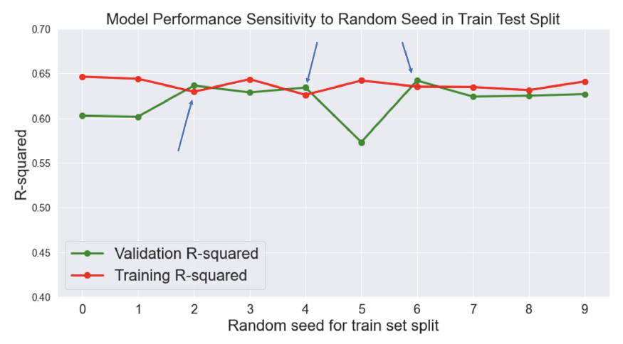
• A better validation set score than the training set score (Notes from link):
  • You don’t have that much data and it’s luck.
    • Can be diagnosed by changing the seed (random_state in py) in data split function
      
  • Gap between them shrinks over time
    • May be do to regularization (if it’s being used).
    • During validation and testing, your loss function only comprises prediction error
  • Gap between them stays the same and training loss has fluctuations
    • DL: dropout is only applicable during the training process, so it only affects training loss
  • Validation loss lower than training loss at first but has similar or higher values later on
    • DL: Training loss is calculated during each epoch, but validation loss is calculated at the end of each epoch
• Compare Training vs Test

  • Example: {gt} table, {yardstick} forecast metrics

    bind_rows(
      yardstick::mape(rf_preds_train, Sale_Price, .pred),
      yardstick::mape(rf_preds_test, Sale_Price, .pred)
    ) %>% 
      mutate(dataset = c("training", "holdout")) %>% 
      gt::gt() %>% 
      gt::fmt_number(".estimate", decimals = 1)

Regression

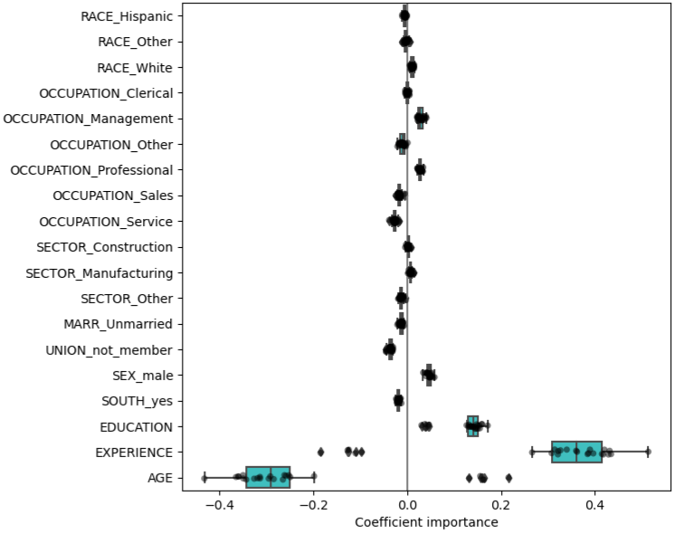
• For prediction, if coefficients vary significantly across the test folds their robustness is not guaranteed (see coefficient boxplot below), and they should probably be interpreted with caution.
  

  • Boxplots show the variance of the coefficient across the folds of a repeated 5-fold cv.
  • The “Coefficient importance” in the example is just the coefficient value of the standardized variable in a ridge regression
  • Note outliers beyond the whiskers for Age and Experience
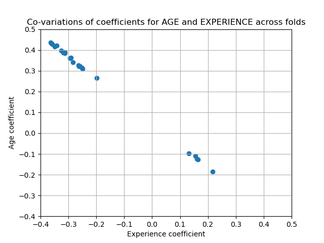
    • In this case, the variance is caused by the fact that experience and age are strongly collinear.
  • Variability in coefficients can also be explained by collinearity between predictors
    
  • Perform sensitivity analysis by removing one of the collinear predictors and re-running the CV. Check if the variance of the variable that was kept has stabilized (e.g. fewer outliers past the whiskers of a boxplot).