Regularized
Misc
- {BoomSpikeSlab} - MCMC for Spike and Slab Regression
- Spike and slab regression is Bayesian regression with prior distributions containing a point mass at zero. The posterior updates the amount of mass on this point, leading to a posterior distribution that is actually sparse, in the sense that if you sample from it many coefficients are actually zeros. Sampling from this posterior distribution is an elegant way to handle Bayesian variable selection and model averaging.
- {ScaleSpikeSlab} - Scalable Spike-and-Slab
- A scalable Gibbs sampling implementation for high dimensional Bayesian regression with the continuous spike-and-slab prior.
- For variable selection, the BSS prior seems to work best with Bayesian Model Averaging (BMA) (paper)
- Also see Feature Selection >> Basic >> Bayesian Model Averaging (BMA)
- {FastKRR} - Kernel Ridge Regression using ’RcppArmadillo
- Parallel execution with OpenMP where available
- Sequential-testing cross-validation that identifies competitive hyperparameters without exhaustive grid search.
- Three scalable approximations—Nyström, Pivoted Cholesky, and Random Fourier Features—allowing analyses with substantially larger sample sizes than are feasible with exact KRR
- Integrates with the {tidymodels} ecosystem via the ‘parsnip’ model specification ‘krr_reg’
- {glmnet} - OG, handles families: Gaussian, binomial, Poisson, probit, quasi-poisson, and negative binomial GLMs, along with a few other special cases: the Cox model, multinomial regression, and multi-response Gaussian.
- {grpnet} - Group Elastic Net Regularized GLMs and GAMs
- Uses lm and glm syntax. Applies regularization penalty (LASSO , MCP, or SCAD) by group variable
- Gaussian, Binomial, Poisson, Multinomial, Negative Binomial, Gamma, and Inverse Gaussian
- {hierNest} - Penalized Regression with Hierarchical Nested Parameterization Structure
- {hspliable} (Paper) - Bayesian pliable LASSO with horseshoe prior
- The pliable lasso model is a sparse model with sparse interaction effects. This package extends the model to GLMs. The Bayesian implementation also makes uncertainty estimation possible.
- Handles missing responses as latent variables, which allows them to derive full conditional distributions in the case of Gaussian observations
- {Multi-Layer-Kernel-Machine} - Multi-Layer Kernel Machine (MLKM) is a Python package for multi-scale nonparametric regression and confidence bands. The method integrates random feature projections with a multi-layer structur
- A fast implementation of Kernel Ridge Regression (KRR) (sklearn) which is used for non-parametric regularized regression.
- Paper: Multi-Layer Kernel Machines: Fast and Optimal Nonparametric Regression with Uncertainty Quantification
- {robustHD}: Robust methods for high-dimensional data, in particular linear model selection techniques based on least angle regression and sparse regression
- In {sklearn} (see Model building, sklearn >> Algorithms >> Stochaistic Gradient Descent (SGD)), the hyperparameters are different than in R
- lambda (R) is alpha (py)
- alpha (R) is 1 - L1_ratio (py)
- {SLOPE} - Lasso regression that handles correlated predictors by clustering them
- {spexvb} - Parameter Expanded Variational Bayes for High-Dimensional Linear Regression
- Utilizes spike-and-slab priors to perform simultaneous estimation and selection
- {uniLasso} - Univariate-Guided Sparse Regression (See Lasso >> uniLasso for details)
- Functions for cross-validation and uniLasso polish. Works with utility functions in {glmnet}
- Also see
- Mathematics, Linear Algebra >> Misc >> Packages >> {sparsevctrs}
- Can create a sparse matrix for glmnet
- Mathematics, Linear Algebra >> Misc >> Packages >> {sparsevctrs}
- Regularized Logistic Regression is most necessary when the number of candidate predictors is large in relationship to the effective sample size 3np(1−p) where p is the proportion of Y=1 Harrell
- If using sparse matrix, then you don’t need to normalize predictors
- Preprocessing
- Standardize numerics
- Dummy or
factorcategoricals - Remove NAs,
na.omit
- Papers
- Predictive Performance Comparison between Logistic LASSO and Ridge
- In general, Ridge outperforms LASSO unless the data are noisy
- Small n and \(\le\) 10 Events per Variable (EPV) \(\rightarrow\) Bad Performance
- Large \(n\) and 10 EPV \(\rightarrow\) Reasonable Performance
- Large \(n\) and \(\gt\) 30 EPV \(\rightarrow\) Penalization effects are small
- Between 10 to 30 EPV \(\rightarrow\)
- Binary prediction models perform worse continuous prediction models
- Think this refers to the dreaded dichotomization of continuous response variables.
- Performance depends on the size of \(n\)
- Binary prediction models perform worse continuous prediction models
- A completely balanced multinomial outcome variable performs worse than a slightly unbalanced one.
- Good performance for balanced multinomial variables requires large EPVs
- At \(\gt\) 50 EPV, performance doesn’t improve much
- Variable Selection
- For Inference, only Adaptive LASSO is capable of handling block and time series dependence structures in data
- See A Critical Review of LASSO and Its Derivatives for Variable Selection Under Dependence Among Covariates
- “We found that one version of the adaptive LASSO of Zou (2006) (AdapL.1se) and the distance correlation algorithm of Febrero-Bande et al. (2019) (DC.VS) are the only ones quite competent in all these scenarios, regarding to different types of dependence.”
- There’s a deeper description of the model in the supplemental materials of the paper. I think the “.1se” means it’s using the lambda.1se from cv.
- lambda.1se : largest value of λ such that error is within 1 standard error of the cross-validated errors for lambda.min.
- see lambda.min, lambda.1se and Cross Validation in Lasso : Binomial Response for code to access this value.
- lambda.1se : largest value of λ such that error is within 1 standard error of the cross-validated errors for lambda.min.
- Re the distance correlation algorithm (it’s a feature selection alg used in this paper as benchmark vs LASSO variants)
- “the distance correlation algorithm for variable selection (DC.VS) of Febrero-Bande et al. (2019). This makes use of the correlation distance (Székely et al., 2007; Szekely & Rizzo, 2017) to implement an iterative procedure (forward) deciding in each step which covariate enters the regression model.”
- Starting from the null model, the distance correlation function, dcor.xy, in {fda.usc} is used to choose the next covariate
- guessing you want large distances and not sure what the stopping criteria is
- algorithm discussed in this paper, Variable selection in Functional Additive Regression Models
- Harrell is skeptical. “I’d be surprised if the probability that adaptive lasso selects the”right” variables is more than 0.1 for N < 500,000.”
- See A Critical Review of LASSO and Its Derivatives for Variable Selection Under Dependence Among Covariates
- For Inference, only Adaptive LASSO is capable of handling block and time series dependence structures in data
Concepts
- Shrinking effect estimates turns out to always be best
- OLS is the Best Linear Unbiased Estimator (BLUE), but being unbiased means the variance of the estimated effects is large from sample to sample and therefore outcome variable predictions using OLS don’t generalize well.
- If you predicted y using the sample mean times some coefficient, it’s always(?) the case that you’ll have a better generalization error with a coefficient less than 1 (shrinkage).
- Regularized Regression vs OLS
- As N ↑, standard errors ↓
- regularized regression and OLS regression produce similar predictions and coefficient estimates.
- As the number of covariates ↑ (relative to the sample size), variance of estimates ↑
- regularized regression and OLS regression produce much different predictions and coefficient estimates
- Therefore OLS predictions are usually fine in a low dimension world (not usually the case)
- As N ↑, standard errors ↓
- Model Equation
\[ \text{argmin}\; \mathcal{L}(\lambda, \alpha) = \frac{1}{2n} \sum_{i=1}^n (y_i - \hat y_i)^2 + \lambda(\frac{1}{2}(1-\alpha)\;||\hat\beta||_2^2\; + \alpha \; ||\hat \beta||_1) \]- \(\lambda\) : The penalization factor
- \(\alpha = 1\) : LASSO
- \(\alpha = 0\) : Ridge
- \(0 \lt \alpha \lt 1\) : Elastic Net
- \(||\hat \beta||_2^2\) : The sum of squared coefficients. The L2 norm has been squared, so the square root isn’t taken.
- When \(\alpha = 0\), the L2 norm is applied.
- \(||\hat \beta||_1\): The sum of the absolute value of coefficients — i.e. L1 norm.
- When \(\alpha = 1\), the L1 norm is applied.
Ridge
- The regularization reduces the influence of correlated variables on the model because the weight is shared between the two predictive variables, so neither alone would have strong weights. This is unlike Lasso which just drops one of the variables (which one gets dropped isn’t consistent).
- Linear transformations in the design matrix will affect the predictions made by ridge regression.
Lasso
- When lasso drops a variable, it doesn’t mean that the variable wasn’t important.
- The variable, \(x_1\), could’ve been correlated with another variable, \(x_2\), and lasso happens to drop \(x_1\) because in this sample, \(x_2\), predicted the outcome just a tad better.
Adaptive LASSO
.png)
- Purple dot indicates that it’s a weighted (\(w_j\)) version of LASSO
- Green checkmark indicates it’s optimization is a convex problem
- Better Selection, Bias Reduction are attributes that it has that are better than standard LASSO
- Weighted versions of the LASSO attach the particular importance of each covariate for a suitable selection of the weights. Joint with iteration, this modification allows for a reduction of the bias.
- Zhou (2006) say that you should choose your weights so the adaptive Lasso estimates have the Oracle Property:
- You will always identify the set of nonzero coefficients…when the sample size is infinite
- The estimates are unbiased, normally distributed, and the correct variance (Zhou (2006) has the technical definition)…when the sample size is infinite.
- To have these properties, \(w_j = \frac{1}{|\hat\beta_j|^q}\), where \(q > 0\) and \(\hat\beta_j\) is an unbiased estimate of the true parameter, \(\beta\)
- Generally, people choose the Ordinary Least Squares (OLS) estimate of \(\beta\) because it will be unbiased. Ridge regression produces coefficient estimates that are biased, so you cannot guarantee the Oracle Property holds.
- In practice, this probably doesn’t matter. The Oracle Property is an asymptotic guarantee (when \(n \rightarrow \infty\)), so it doesn’t necessary apply to your data with a finite number of observations. There may be scenarios where using Ridge estimates for weights performs really well. Zhou (2006) recommends using Ridge regression over OLS when your variables are highly correlated.
- Generally, people choose the Ordinary Least Squares (OLS) estimate of \(\beta\) because it will be unbiased. Ridge regression produces coefficient estimates that are biased, so you cannot guarantee the Oracle Property holds.
- Zhou (2006) say that you should choose your weights so the adaptive Lasso estimates have the Oracle Property:
- See article, Adaptive LASSO, for examples with a continuous, binary, and multinomial outcome
uniLasso
- Univariate-Guided Sparse Regression by Sourav Chatterjee, Trevor Hastie, and Robert Tibshirani (See Misc >> Packages >> {uniLasso}
- A more stable and easier to interpret version of LASSO
- Ensures the signs of the final coefficients match the signs of their univariate coefficients (or are set to zero)
- Standard LASSO can sometimes assign a negative coefficient to a variable that has a positive univariate correlation due to correlations with other predictors. Such sign flips can be confusing and make a model less credible.
- Uses the magnitude of the univariate coefficients to guide the final model. Features that have a stronger relationship with the outcome individually are encouraged to have larger coefficients in the final model.
- This ensures that the final model reflects the “relative importance” of predictors as seen in the raw data. (i.e. the coefficient magnitude reflects variable importance)
- In uniLasso, larger coefficients are shrunk less than smaller ones. This means that strong signals are preserved more faithfully in the final model compared to standard Lasso, where they might be overly penalized.
- Outperformed LASSO, especially in choosing fewer, more meaningful variables without sacrificing accuracy.
- uniLasso was shown to have a much lower false positive rate than LASSO, meaning it is less likely to include irrelevant “spurious features” in the final model.
- Can be extended beyond basic regression to more complex settings, including models used for analyzing survival times and other common statistical frameworks.
- Overview
- It looks at how each variable relates to the outcome by itself, and it keeps track of whether the relationship is positive or negative.
- Then, it combines these relationships into a final model.
- uniLasso Polish - A postprocessing of uniLasso in which the lasso is applied to the uniLasso residuals.
- Adaptive lasso is equivalent to uniLasso using non-LOO estimates and no sign constraints
- Algorithim
For \(j = 1, 2, \ldots, p\) compute the univariate intercepts and slopes \((\hat{\beta}_{0j}, \hat{\beta}_j)\) and their leave-one-out (LOO) counterparts \((\hat{\beta}_{0j}^{-i}, \hat{\beta}_j^{-i})\), \(i = 1, \ldots, n\).
Fit the lasso—with an intercept, no standardization, and nonnegativity constraints—to target \(y\) and the univariate LOO fits as features
\[ \text{minimize}_{\theta} \left\{ \frac{1}{n} \sum_{i=1}^{n} \left( y_i - \theta_0 - \sum_{j=1}^{p} (\hat{\beta}_{0j}^{-i} + \hat{\beta}_j^{-i} x_{ij}) \theta_j \right)^2 + \lambda \sum_{j=1}^{p} \theta_j \right\} \]
- Subject to \(\theta_j \geq 0 \, \forall j > 0\).
The final model can be written as \(\hat{\eta}(x) = \hat{\gamma}_0 + \sum_{j=1}^{p} \hat{\gamma}_j x_j\), with \(\hat{\gamma}_j = \hat{\beta}_j \hat{\theta}_j\), and \(\hat{\gamma}_0 = \hat{\theta}_0 + \sum_{\ell=1}^{p} \hat{\beta}_{0\ell} \hat{\theta}_\ell\).
- “we do not standardize the features before applying the nonnegative lasso in Step 2;” So I’m guessing there’s no preprocessing except maybe one-hot encoding categorical variables.
Firth’s Estimator
Penalized Logistic Regression estimator
For sample sizes less than around n = 1000 or sparse data, using Firth Estimator is recommended
Misc
- Notes from
- Packages
- {brglm2} - Estimation and inference from generalized linear models using explicit and implicit methods for bias reduction
- {logistf} - Includes FLIC and FLAC extensions; uses profile penalized likelihood confidence intervals which outperform Wald intervals; includes a function that performs a penalized likelihood ratio test on some (or all) selected factors
emmeans::emmeansis supported
- Invariant to linear transformations of the design matrix (i.e. predictor variables) unlike Ridge Regression
- While the standard Firth correction leads to shrinkage in all parameters, including the intercept, and hence produces predictions which are biased towards 0.5, FLIC and FLAC are able to exclude the intercept from shrinkage while maintaining the desirable properties of the Firth correction and ensure that the sum of the predicted probabilities equals the number of events.
- {brglm2} works easily with multiply imputed data but doesn’t produce corrected predicted probabilities. {logistf} can produce corrected predicted probabilities, but doesn’t easily work with multiply imputed data. (source)
Penalized Likelihood
\[ L^*(\beta\;|\;y) = L(\beta\;|\;y)\;|I(\beta)|^{\frac{1}{2}} \]
Equivalent to penalization of the log-likelihood by the Jeffreys prior
\(I(\beta)\) is the Fisher information matrix, i. e. minus the second derivative of the log likelihood
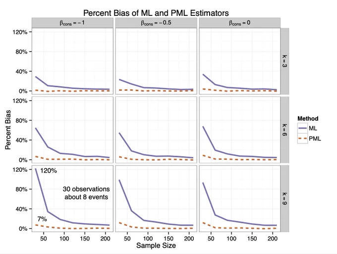
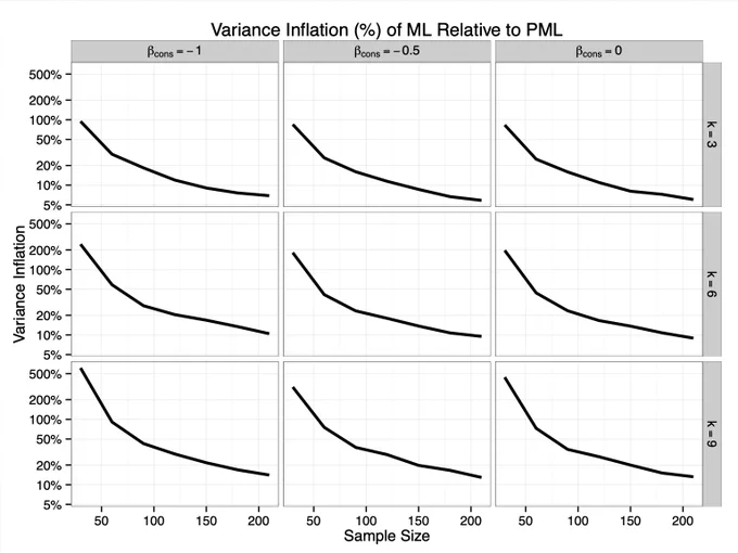
Maximum Likelihood vs Firth’s Correction
Bias
Variance
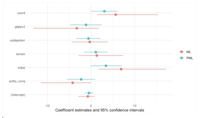
Coefficient and CI bar comparison on a small dataset (n = 35, k = 7)
Limitations
- Relies on maximum likelihood estimation, which can be sensitive to datasets with large random sampling variation. In such cases, Ridge Regression may be a better choice as it provides some shrinkage and can stabilize the estimates by pulling them towards the observed event rate.
- Less effective than ridge regression in datasets with highly correlated covariates
- For the Firth Estimator, the Wald Test can perform poorly in data sets with extremely rare events.