Analysis
Misc
- Also see
- Packages
- {causalWins} - Compute the Causal Win Ratio Using Nearest Neighbor Matching
- {CEACT} - Designed to facilitate the economic evaluation of healthcare interventions in randomized trials. It offers a suite of functions for estimating and visualizing core cost-effectiveness metrics, including:
- Incremental Cost-Effectiveness Ratios (ICER)
- Cost-effectiveness planes
- Cost-effectiveness acceptability curves (CEAC)
- Net monetary benefit (NMB) metrics
- {evalHTE} - Provides various statistical methods for evaluating heterogeneous treatment effects (HTE) in randomized experiments
- Estimate uniform confidence bands for estimation of the group average treatment effect sorted by generic machine learning algorithms (GATES)
- Tools to identify a subgroup of individuals who are likely to benefit from a treatment the most “exceptional responders” or those who are harmed by it.
- {pmrm} - A progression model for repeated measures (PMRM) is a continuous-time nonlinear mixed-effects model for longitudinal clinical trials in progressive diseases.
- Unlike mixed models for repeated measures (MMRMs), which estimate treatment effects as linear combinations of additive effects on the outcome scale, PMRMs characterize treatment effects in terms of the underlying disease trajectory
- Resources
- Introduction to Bayes for Evaluating Treatments (Harrell)
- Solomon Kurz posts for analyzing RCTs
- Heiss’s basic tutorial - Randomized controlled trials (RCTs)
- Papers
- Numerical validation as a critical aspect in bringing R to the Clinical Research
- Slides that show various discrepancies between R output and programs like SAS and SPSS and their solutions.
- Procedure for adopting packages into core analysis procedures (i.e. popularity, documentation, author activity, etc.)
- Numerical validation as a critical aspect in bringing R to the Clinical Research
- Spline — don’t bin continuous, baseline, adjustment variables, where “baseline” means the patients measurements before treatment. Lack of fit will then come only from omitted interaction effects. (Harrell)
- e.g.: if older males are much more likely to receive treatment B than treatment A than what would be expected from the effects of age and sex alone, adjustment for the additive propensity would not adequately balance for age and sex.
- Also see
- Making causal statements from RCTs
- “relative efficacy,” “cause,” “impact,” or “resulted in” when used to describe the effect from an RCT are interchangable
- Example: “Under prior P, Treatment B probably (0.949) causes a reduction in blood pressure relative to treatment A, and it probably (0.83) causes at least a 5 mmHg reduction.” (Harrell)
- Analysis of a two armed trial comparing a treatment to placebo:
- Questions
- Was there a treatment effect in this trial?
- What was the ATE of this trial?
- Was the treatment effect identical for all patients in the trial?
- What was the treatment effect for the different subgroups of the trial?
- What will the treatment effect be when used more generally (outside the trial)?
- Strategies
- (Predictive) adjustment variables (e.g. Age) are good to help answer Q1 & Q2
- Interactions (group_cat ⨯ treatment) could help answer Q3 and Q4.
- Q5 is about external validity (see Diagnostics, Classification >> Terms)
- Questions
- Analysis shouldn’t only include Intent-to-Treat effects
- To adequately guide decision making by all stakeholders, report estimates of both the intention-to-treat effect and the per-protocol effect, as well as methods and key conditions underlying the estimation procedures.
- “Intent-to-treat analysis makes sense from a public health point of view if it closely reflects the actual medical practice. But from a patient point of view of making a decision regarding treatment, the actual treatment is more meaningful than intent-to-treat. So, when the two estimates differ considerably, it seems to me that they should both be reported – or, at least, the data should be provided that would allow both analyses to be done.” Lehman from Gelman blog post
- “The correct model models the 4 groups and the conditional probability to be in the 4 groups as a function of pre-treatment covariates, including both psychological covariates, cultural covariates, as well as symptomatic and disease progression knowledge.” Lakeland
- Analysis of substudies must be separate
- Example: Study Effects: 2 Studies with the same treatment (Lumiracoxib), but different controls (ibuprofen, naproxen) (article)
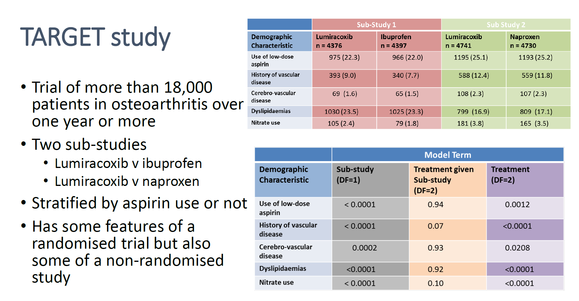
- Cells are p-values
- Bottom table shows when a “Sub-Study” indicator is used as a model term (“Treatment given Sub-study”) vs not used (“Treatment”), the p-values for all the “Demographic Characteristic” variables lose significance.
- Example: Study Effects: 2 Studies with the same treatment (Lumiracoxib), but different controls (ibuprofen, naproxen) (article)
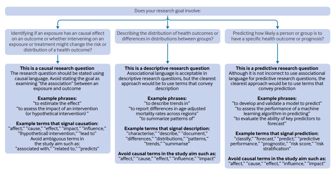
- Appropriate language for results based on the research question (source)
Terms
Estimand - A description of the exact treatment effect a study aims to quantify for a given outcome. They describe how outcomes would change between different treatment strategies for the same set of participants.
Estimator - The statistical method used to compute the estimate of the treatment effect.
Estimate - The numerical value computed by the estimator. For example, in a study reporting an estimated mean difference between groups of −0.7 (95% confidence interval −0.3 to −1.1), the value −0.7 is the estimate.
Interim Analysis - An analysis of data that is conducted before data collection has been completed.
- Clinical trials are unusual in that enrollment of subjects is a continual process staggered in time. If a treatment can be proven to be clearly beneficial or harmful compared to the concurrent control, or to be obviously futile, based on a pre-defined analysis of an incomplete data set while the study is on-going, the investigators may stop the study early.
Compliance
- Refers to how observations respond to treatment.
- Full compliance with treatment means that all units to whom a program (i.e. treatment) has been offered actually enroll, and none of the control (aka comparison) units receive the program
- Exclusion of some randomized subjects can be justified (such as patients who were deemed ineligible after randomization or certain patients who never started treatment) when analyzing the results of an experiment.
- Types
- Always-Takers: A person who receives the treatment regardless of the assignment (or instrument in IV).
- Never-Takers: A person who never receives the treatment regardless of the assignment (or instrument in IV).
- Compliers: A person who receives the treatment only when assigned to the treatment group (or when the instrument compels them to).
- Defiers: A person who receives the treatment only when they are NOT assigned to the treament group (or the instrument does not compel them to). They always do the opposite of what the assignment mechanism instructs them to do (assholes). Usually a reasonable assumption to make that there are none in your (quasi-) experiment, but it can only be made based on intuition
- Example: Receiving additional years of Education is the treatment; whether an educational Reform was implemented in their region is the instrument
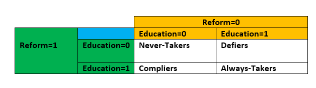
- A person who decides to stay in school regardless of whether there’s a government policy to do so would be an Always-Taker (Education=1, regardless of Reform)
- Compliance Modeling (Lakeland thread)
- Model how people make the decision to adhere to the randomization or not (“Person makes decision about actual treatment” step)
- Realistic Model: Enroll person \(\rightarrow\) Randomize to treatment group \(\rightarrow\) Person makes decision about actual treatment \(\rightarrow\) Actual treatment occurs \(\rightarrow\) Outcomes observed
- ITT effect by itself is misleading
- Suppose you did a mouse experiment and randomized mice to different surgeries and then told the surgeons to do the surgery they were randomized to unless they see conditions A,B,C in which case do a different surgery, and then analyzed via intention to treat. That would just be disingenuous. The fact that we don’t know a precise rule for adherence doesn’t mean adherence isn’t part of the question. So build a probabilistic rule for adherence
- Highlights a source of uncertainty which should then increase the uncertainty in the final analysis, but would not be included in the ITT or any other frequentist analysis
- Example: Prostate Cancer
Pretreatment Survey
- You’re trying to understand the patient’s state-of-mind.
- Questions:
- What is your age?
- What is your biological sex?
- What race do you identify as (set of choices)?
- What religious affiliation do you affiliate most with … (set of choices)?
- On the following scale rate the discomfort that your condition causes… 0,1,2,3,4,5,6 with some text descriptors from “none” to “severe discomfort”
- What is your education level (from some grade school to PhD, and a check mark for whether it’s a biology/medicine related degree)
- Check all that apply: what are the primary motivations for entering the study (things like “to get free treatment” and “to improve the state of knowledge about the disease” and various other things)
- What is your income level?
- Do you have insurance that would cover this treatment outside the study? What is the level of coverage?
- What is your level of concern about having surgery? (from zero to “I am very nervous about having surgery”)
- What is your level of concern about potential side effects (similar scale)?
- Which side effects are you concerned about (check boxes)?
- What are your existing thoughts about watchful waiting (0 I believe it is not right for me, up to 6 watchful waiting is my currently preferred treatment)?
- What is your current belief about the severity of your condition: similar?
- What is your current belief about the aggressiveness of your condition: similar?
- What is your current belief about metastatic tumors?: 0… I have no reason to believe… 6 … I have medical biopsy proving metastatic
Bayesian Procedure
- Now, hypothesize at least the *direction* that each of these affects the probability of compliance with surgery assignment, and with watchful waiting assignment.
- Place a prior over coefficients of each one with bias towards the direction hypothesized in a logistic regression with nonlinear response on any variables that may seem appropriate.
- Now, hypothesize the direction with which some subset of these predicts actual aggressiveness of the underlying condition, for example using the patients own beliefs, using the reported level of symptoms, using info about metastatic condition, etc.
- Place prior over coefficients in a hidden variable model for severity… again with nonlinear response if necessary.
- Collect data
- Posterior distribution of parameters…
Model:
\[\begin{aligned} \mbox{adherence} \;\sim\; &\mbox{Binomial}(\mbox{inv\_logit}( \\ &k \times \mbox{symptom\_severity} \times \mbox{assigned\_monitoring} + \mbox{random\_individual\_factor}\\ &)) \end{aligned}\]
- With random_individual_factor having a group level prior distribution gets an estimate of the probability of adherence
- So you can fit probability of good outcome based on adherence with symptom_severity informing, telling you something about whether outcomes are due to selection or severity.
- Model how people make the decision to adhere to the randomization or not (“Person makes decision about actual treatment” step)
Risk
- Also see
- Regression, Ordinal >> Proportional Odds >> Examples for calculations of Risk Differences and Risk Ratios
- Regression, Logistic >> Log Binomial who’s exponentiated coefficients are Risk Ratios
- Recommended metrics to be reported for medical studies (Harrell). This is perhaps generalizable to any RCT with a binary outcome.
- The distribution of Risk Difference (RD)
- Covariate-Adjusted OR
- Adjusted marginal RD (mean personalized predicted risk as if all patients were on treatment A minus mean predicted risk as if all patients were on treatment B) (emmeans?)
- Median RD
- The best information to present to the patient is the estimated individualized risk of the bad outcome separately under all treatment alternatives. That is because patients tend to think in terms of absolute risk, and differences in risks don’t tell the whole story (Harrell)
- A risk difference (RD, also called absolute risk reduction) often means different things to patients depending on whether the base risk is very small, in the middle, or very large.
- Risk Difference (aka Absolute Risk)((aka Prevalence Difference in cross-sectional studies) is important when probabilities of an event are high. Using the Risk Ratio in this circumstance has a tendency to downplay the difference.
- Example: 95% chance for event A vs 90% chance of event B
- Risk Ratio: 0.95/090 says event A is 1.06 times more likely
- Risk Difference: 0.95 - 0.90 says Event A is 5% more likely
- Example: 95% chance for event A vs 90% chance of event B
- Risk Ratios (aka Relative Risk) are more intuitive than odds ratios.
- Most helpful when wanting to understand the relative impact of a condition (i.e. when predictor = category A vs Category B).
- Most informative when probabilities are low (small differences can mean substantial effects)
- Example: 1% chance of event A and 2% chance of event B
- Risk Difference: 0.02 - 0.01 = 1% difference
- Risk Ratio: 0.02/0.01 = 2 (or twice the risk!)
- Risk Ratios and Risk Diffference may have substantially different p-values. Different tests and scales are involved.
Effects
Packages
- {transportr} - Transporting Intervention Effects from One Population to Another
- {RobinCar2} - Performs robust estimation and inference when using covariate adjustment and/or covariate-adaptive randomization in randomized controlled trials.
- {postcard} - Tools for accurately estimating marginal effects using plug-in estimation with GLMs, including increasing precision using prognostic covariate adjustment.
- Similar to a glm, but requires these specifications:
- The randomisation variable in data, usually being the (name of) the treatment variable
- The randomisation ratio - the probability of being allocated to group 1 (rather than 0)
- As a default, a ratio of 1’s in data is used
- An estimand function
- As a default, the function takes the average treatment effect (ATE) as the estimand
- Similar to a glm, but requires these specifications:
Resources
- Potential Outcomes, ATEs, and CATEs
- Complier Average Treatment Effects - Heiss tutorial for ITT and CACE
Comparison
.png)
- ATE is for the whole population (he should’ve had the arrow coming out of the word, population, or the edge of the circle)
- Circle is split into half: treatment (upper left, yellow), control/comparison (bottom right, pink)
- ATT is for treated (treated compliers, always takers, treated defiers)
- ATU is for control/comparison (non-treated compliers, never takers, non-treated defiers)
- LATE is for treated compliers
- CATE is for a subset of the population (e.g. men)
Heterogeneous Treatment Effect (HTE) - Also called differential treatment effect, includes difference of means, odds ratios, and Hazard ratios for time-to-event outcome vars
- Also see Dahly article for links to avoid pitfalls when using this effect
- Ascertaining subpopulations for which a treatment is most beneficial (or harmful) is an important goal of many clinical trials.
- Outcome heterogeneity is due to wide distributions of baseline prognostic factors. When strong risk factors exist, there is hetergeneity in the outcome variable.
- Solution: add baseline predictors to your model that account for these strong risk factors.
- Heterogeneity of Treatment Effects - The degree to which different treatments have differential causal effects on each unit.
- Examples
- The effect of attending college on earnings differs across students
- The effect of a state-wide smoking ban on smoking rates varies across states
Intention-to-Treat (ITT) - estimates the difference in outcomes between the units assigned to the treatment group and the units assigned to the control (aka comparison group in quasi-experiments) group, irrespective of whether the units assigned to the treatment group actually receive the treatment. An intention-to-treat analysis is not feasible if trial participants are lost to follow-up
- Potential solution: weighted average of the outcomes of participants and non-participants in the treatment group compared with the average outcome of the control group
- Example: Doctor tells everyone in a treatment group to go home and exercise for an hour per day and tell the control group nothing.
- After a month, if you just compare the difference in mean blood pressures between the two groups, you get the intention to treat estimator
- Doesn’t tell you the causal effect of exercise on blood pressure, but the causal effect of telling people to exercise on blood pressure.
- This estimate would be smaller than the treatment effect of exercise per se, as only a (small!) fraction of people in the treatment group would completely follow the treatment
Modified Intention-to-Treat (mITT) - No ineligible users. This applies to cases where we detect the ineligibility after assignment, but the eligibility criteria are based on factors that could have been known before the experiment. Hence, it should be safe to exclude the ineligible users after the fact
- e.g. bots and existing users should increase the observed effect size, but not change the preferred variant.
Modified Intention-to-Treat No Crossovers (mITTnc). If we have a mechanism to detect some crossovers, excluding them and comparing the results to the intention-to-treat analysis may uncover implementation bugs.
- Crossovers are users that experience both the treatment and control exposures or (unintentionally) more than one treatment
- It’s worth noting that crossovers shouldn’t occur in cases where we can uniquely identify users at all stages of the experiment – it is a problem that is more likely to occur when dealing with anonymous users.
- As such, and given the inability to detect all crossovers, A/B experiments should be avoided when users are highly motivated to cross over.
- Example: displaying different price levels based on anonymous and transient identifiers like cookies is often a bad idea.
Average Treatement Effect (ATE) - Expected causal effect of the treatment across all individuals in the study population
AKA Sample Average Treatment Effect (SATE) which is the effect of the treatment variable in the analysis of a RCT. Although, RCT results aren’t technically generalizable to a larger population, so the participants in the study could be considered the population in this regard.
AKA Population Average Treatment Effect (PATE)
- Seen this term used in a propensity score matching paper.
For a linear model estimate, \(Y_i = \beta_0 + \beta_1 X_i + u_i\)
\[\begin{aligned} \beta_1 &= \mbox{ATE} \\ &= \mathbb{E}[Y \;|\;X = 1] − \mathbb{E}[Y \;|\;X = 0] \\ &= \mathbb{E}[\beta_1,\;i ] \end{aligned}\]
- Which is the Average effect of a unit change in \(X\)
Conditional Average Treatment Effect (CATE) - ATE for a subgroup
\[\text{CATE} = \mathbb{E}(Y \;|\: A = 1, X = x) - \mathbb{E}(Y \;|\: A = 0, X = x)\]
- Where \(A\) is the treatment and \(X\) are covariates
- Coefficient for an interaction (i.e. explanatory*treatment)
- Contains information about treatment heterogeneity across population subgroups, as opposed to the average treatment effect (ATE), which averages treatment effects over the entire population
Average Treatment Effect on the Treated (ATT) - Expected causal effect of the treatment for individuals in the treatment group
\[\begin{aligned} ATT &= E[\delta \;|\; D = 1] \\ &= E[Y^1 − Y^0 \;|\; D = 1] \\ &= E[Y^1 \;|\; D = 1] − E[Y^0 \;|\; D = 1] \end{aligned}\]
- Where \(\delta\) is the individual-level causal effect of the treatment and \(D\) is the treatment
- In the ideal scenario of a randomized control trial (RCT) (commonly violated in observational studies), ATE equals ATT because we assume that:
- The baseline of the treatment group equals the baseline of the control group (layman terms: people in the treatment group would do as bad as the control group if they were not treated) and
- The treatment effect on the treated group equals the treatment effect on the control group (layman terms: people in the control group would do as good as the treatment group if they were treated).
- ATT should be used instead of ATE when there’s extreme imbalance between covariate criteria of treated vs control/comparison groups (e.g. quasi-experiment)
.png)
- Also see Econometrics, General >> Propensity Scoring Matching
- Overlap plot or balance plot from video
- {cobalt} may provide a way generate these
- y-axis: count, x-axis: covariate, color: treatment
- The range of x covered by blue (treatment) is much smaller than the range of x covered by red (control), therefore ATT might be a better choice of estimated effect
Target Average Treatment Effect (TATE) - A causal estimand that measures the average impact of a treatment on a specific, distinct target population, often generalizing results from a controlled trial (source) to a real-world setting. (i.e. Focuses on the generalizability or transportability of an effect to an external population)
- Packages
- {ROOT} - A general functional optimization framework for learning interpretable binary weight functions, represented as sparse decision trees
- Introduces a refined estimand, the Weighted Target Average Treatment Effect (WTATE), defined over the subset of the population that is sufficiently represented.
Units are either included (\(w(X)=1\)) or excluded (\(w(X)=0\)) according to learned tree-structured rules.
The loss function is designed to minimize the variance of the estimator while retaining as much of the target population as possible.
- Introduces a refined estimand, the Weighted Target Average Treatment Effect (WTATE), defined over the subset of the population that is sufficiently represented.
- {ROOT} - A general functional optimization framework for learning interpretable binary weight functions, represented as sparse decision trees
- It addresses, via weighting or modeling, how treatment effects differ when the target population’s characteristics (covariates) differ from the trial sample
- Estimates the effect of a treatment, intervention, or policy on a population that differs from the experimental sample, such as applying clinical trial results to a broader, real-world patient group (External Validity?)
- Estimation approaches:
- Weighting Methods: Adjusting the study sample so its characteristics resemble the target population, often using inverse probability weighting.
- Outcome Modeling: Fitting a flexible model (like Bayesian Additive Regression Trees or Random Survival Forests) to the study data and then using it to predict outcomes for every individual in the target population.
- Doubly Robust Estimators: Combining both weighting and outcome models to provide a more reliable estimate that is accurate if at least one of the models is correctly specified.
- Packages
Local Average Treatment Effect (LATE) - Applies when there is noncompliance in the treatment group, comparison group, or both simultaneously.
- If there is noncompliance in both the treatment and comparison group, then the LATE estimate is valid only for those in the treatment group (who enrolled in the program; i.e. treated) and (who would have not enrolled had they been assigned to the control/comparison group).
- “Who would have not enrolled had they been assigned to the comparison group” is a weird counterfactual
- “Local” indicates that LATE is the average effect for the group known as compliers
- Treatment and Instrument are binary variables
- IV models still valid for treatments and instruments with more than 2 levels, but effect calculation is more complicated
- Calculation (always-takers and defiers are assumed not to exist)
- LATE = (avg potential outcome of compliers who do receive treatment) - (avg potential outcome of compliers who don’t receive treatment)
- The (avg potential outcome of compliers who don’t receive treatment) has to be solved for.
- Given that we know the proportions and outcomes for the compliers and never-takers in our treatment group, you can solve a simple equation for this quantity.
- See video for details
- Think this is the primary estimate of an IV model as well (See Econometrics, General >> Instumental Variables)
- Treatment-on-the-treated (ToT) is simply a LATE in the more specific case when there is noncompliance only in the treatment group. Estimates the difference in outcomes between the units that actually receive the treatment and the comparison group (Seems similar to ATT)
Per-Protocol Effect (PPE) - The effect of receiving the assigned treatment strategies throughout the follow-up as specified in the study protocol
- i.e. The effect that would have been observed if all patients had adhered to the protocol of the RCT
- Alternative to the intention-to-treat effect that is not affected by the study-specific adherence to treatment
- Valid estimation of the per-protocol effect in the presence of imperfect adherence generally requires untestable assumptions
- Approaches below are generally invalid to estimate the per-protocol effect. (G-estimation and instrumental variable methods can sometimes be used to estimate some form of per-protocol effects even in the presence of unmeasured confounders)
- (Biased) Approaches:
As-Treated: Compare the outcomes of those who took treatment (\(A=1\)) and didn’t take the the treatment (\(A=0\)) regardless of their assignment
\[\mbox{Pr}(Y=1 \;|\; A=1) \;-\; \mbox{Pr}(Y=1 \;|\; A=0)\]
Per-Protocol: Compare the outcomes of those who took treatment (\(A=1\)) among those assigned to Treatment (\(Z=1\)) to those who didn’t take the treatment (\(A=0\)) among those assigned to Control (\(Z=0\))
\[\mbox{Pr}(Y=1 \;|\; A=1,\;Z=1) \;-\; \mbox{Pr}(Y=1 \;|\; A=0, \; Z=0)\]
- (Biased) Approaches:
Intercurrent Events
Events that occur post-randomization or post-baseline or post-treatment initiation, which can affect the interpretation of treatment effects.
Notes from The estimands framework: a primer on the ICH E9(R1) addendum
Inclusion of patients involved in intercurrent events pulls the overall treatment effect towards zero, rendering it more difficult to identify a beneficial (or harmful) intervention effect.
(Common) Categories:
- Treatment-modifying Events - Events that affect receipt of the assigned treatment
- Early discontinuation of the study’s treatment and then use of a rescue treatment.
- Wrong dosage
- Received treatment is different from the assigned treatment
- Truncating Events - Events preclude the existence of the outcome
- Death
- e.g. If a patient dies in week 6, then a measurement is not possible in week 12. The week 12 measurement is not considered to be missing data, which implies that it could have been collected but was not.
- Amputation of a limb when the outcome is a symptom score based on that limb
- Miscarriage when the outcome is neonatal birth weight
- In time-to-event settings, truncating events that prevent the outcome of interest from occurring are often referred to as competing events. (See Regression, Survival >> Terms >> Competing Risks)
- Death
- Treatment-modifying Events - Events that affect receipt of the assigned treatment
Examples
- If a patient stops taking a treatment early or receives a different treatment to the one they were meant to or an additional non-study treatment.
- Loss to follow-up, study withdrawal, and missing data frequently occur alongside certain intercurrent events, but they are not themselves intercurrent events.
- The treatment discontinuation affects our interpretation of outcome data, and not the withdrawal from the study.
- Some but not all protocol deviations can also be intercurrent events. Intercurrent event status depends on whether the protocol deviation affects assigned treatment.
- If it does affect assigned treatment (eg, receipt of prohibited drug treatment), the deviation is an intercurrent event
- If it does not affect assigned treatment (eg, failure to take proper informed consent), the deviation usually is not an intercurrent event.
Example: FLO-ELA Trial
- A pragmatic trial comparing two methods of fluid delivery (cardiac output monitor v clinician judgment) in patients undergoing emergency bowel surgery
- Because of the lead-in time required to prepare the intervention, a small delay between randomization and the start of surgery is necessary.
- Some participants in FLO-ELA could have their surgery cancelled after randomization, either because they become too unwell or the underlying issue has resolved itself. Here, cancellation of surgery is an example of an Intercurrent Event.
Mitigation Strategies
Strategy Definition Points to consider Treatment policy The intercurrent event is considered part of the treatment strategy, so outcomes are used whether or not the intercurrent event occurred Cannot be used for truncating intercurrent events, such as death
Can be used to evaluate the intervention if used as part of routine practice, provided that the intercurrent event under consideration would occur in routine practice as well as in the study settingComposite The intercurrent event is incorporated into the outcome definition, and participants who experience the intercurrent event are assigned to a particular outcome value Modifies the endpoint attribute of the estimand
Changes the interpretation of the estimand to include the effect of treatment on the occurrence of the intercurrent event
Different composite estimands could be defined on the basis of the choice of value assigned to the outcome
Should not be used for intercurrent events only affecting one treatment group, because this action involves defining the outcome differently between treatments, which could introduce artificial differencesWhile-on-treatment/while-alive The outcome before the occurrence of the intercurrent event is of interest Modifies the endpoint attribute of the estimand
Different while-on-treatment/while-alive estimands could be defined, depending on which outcomes are used before occurrence of the intercurrent event
This strategy can compare outcomes at different time points between treatment groups, which can make the intervention appear effective (or harmful) even when it has no direct effect on the outcomeHypothetical The outcome pertaining to a hypothetical setting where the intercurrent event would not (or would) occur is of interest Could modify the treatment attribute of the estimand
Multiple hypothetical settings could apply, so the precise hypothetical setting envisaged should be described
How the hypothetical setting would occur should be justified, to ensure that the estimand is well defined and to facilitate critical appraisal of the estimand’s clinical relevancePrincipal stratum The outcome in a subpopulation of patients who would not (or would) experience the intercurrent event is of interest Modifies the population attribute of the estimand
Different principal stratum populations can be defined—for instance, participants who would not discontinue either assigned treatment versus those who would not discontinue if assigned to intervention
Calculating LATE
- Misc
- Experiment
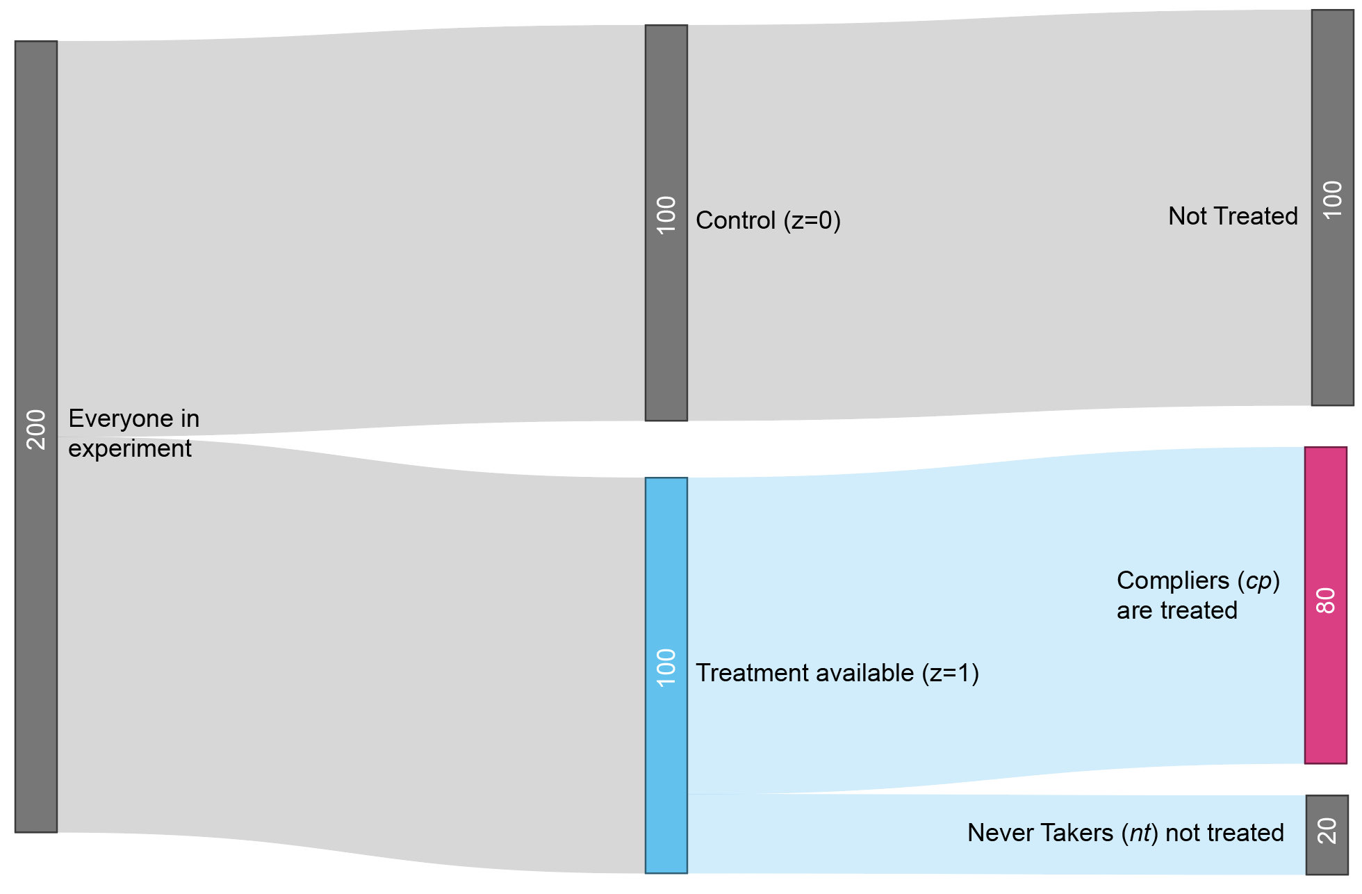
- \(z\) is the treatment availability assignment
- \(\mbox{cp}\) is shorthand for complier, referring to people who complied with the instructions.
- \(Y_{\text{cp},\;z = 1}\) therefore represents the average outcome of the group that actually received treatment, since they were compliers (\(\text{cp}\)) who were randomly assigned to treatment availability (\(z=1\)).
- \(Y_{z = 0}\) represents the average outcome of the control group (\(z=0\)).
- Local Average Treatment Effect (LATE)
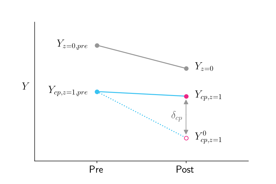
The LATE tells you how much the treatment affects the people who actually got treated
Formula
\[\delta_{\text{cp}} = Y_{\text{cp},\; z=1} - Y^0_{\text{cp},\; z=1}\]
- \(\delta_{\text{cp}}\) is the Local Average Treatment Effect (LATE), since it reflects the impact of the treatment on a particular subpopulation (subpopulation being the compliers who were treated)
- \(Y_{\text{cp},\;z = 1}\) is the average outcome for compliers who were treated
- \(Y^0_{\text{cp},\;z=1}\) is the average outcome for compliers if they hypothetically weren’t treated (counterfactual)
Using substitution and some algebra (See article above for details), the counterfactual part can be avoided and this equation becomes
\[\delta_{\text{cp}} = \frac{Y_{z=1} - Y_{z=0}}{\pi_{\text{cp}}}\]
- \(\pi_{\text{cp}}\) is the fraction of compliers
- Bias within complier group
- Group’s counterfactual outcomes might be different from other groups.
- LATE accounts for that by correctly reporting the impact of the treatment relative to the counterfactual.
- The treatment might be more effective in the complier group than in the never-taker group.
- That bias is unescapable and is known as a heterogenous treatment effect. The way to deal with this bias is to acknowledge it transparently.
- Group’s counterfactual outcomes might be different from other groups.
- If treatment involves more than a single dose, and people can withdraw midway through the program.
- Report the Intention To Treat (ITT) metric, which is the impact of being assigned to treatment (\(Y_{z=1} − Y_{z=0}\)) rather than the impact of being treated.
Change Score Models
Change Scores - Subtract the baseline value of the outcome from the value measured at the end of the study and use that difference for your statistical tests or models.
This is a within-group effect and only should be reported if the between-group effect (i.e. treatment effect) is significant. The between-arm estimate is what’s important. (One simple trick that statisticians hate)
- Regarding significant within-group effect: “Perhaps the improvement was due to the treatment, but maybe it was just the natural progression of the illness (a true improvement occurring with the passage of time), or regression to the mean (a statistical artifact masquerading as improvement).”
- After a null result for the treatment effect, some researchers will muddy the waters by reporting significant within-arm effects.
Misc
- Resources
- Reason: Randomization of participants will result in groups (e.g. treated/control) that are comparable “on average” over many hypothetical trials, at the end of the day, we just have the one trial that we actually ran. And for that one trial there really could be important differences between the groups at baseline that could lead to errors of inference (e.g. concluding the treatment is beneficial when it isn’t).
- Example: A trial for a blood pressure medication that we hope will lower patients’ SBP values. So we set up the trial, recruit some patients and randomize them into two groups. Then we give one group the new medication we are testing, and the other gets standard-of-care. At the end of the study we compare the mean blood pressure of the two groups and find that the active group had a SBP that was 3 mmHg lower, on average, than the values seen in the control group. We might thus conclude that the treatment worked. However, what if it just so happened that the active group also had a similarly lower mean blood pressure (vs the other group) measured at baseline, before the intervention?
- Do not use a change score model to analyze observational data (Paper, Thread)
Example: Change Score Model
\[\begin{aligned} &\mbox{post}_i - \mbox{pre}_i \sim \mathcal{N}(\mu_i, \sigma_\epsilon) \\ &\text{where} \: \mu_i = \beta_0 + \beta_1 \mbox{tx}_i \end{aligned}\]
w1 <-
  glm(data = dw,
      family = gaussian,
      (post - pre) ~ 1 + tx)
Specification
- \(\mbox{post}\), \(\mbox{pre}\) are pre-treatment, post-treatment measurements of the outcome variable
- \(\mbox{tx}\) is the treatment indicator variable
- \(\beta_0\): Population mean for the change in the control group
- Easier to interpret if pre is mean centered
- \(\beta_1\): Parameter is the population level difference in pre/post change in the treatment group, compared to the control group.
- Also a causal estimate for the average treatment effect (ATE) in the population, \(\tau\)
Examples
- Example 1: Pretest-Posttest Between-Person Factorial Design to compare competing theories on depression and suicidal behaviors. (link)
- Example 2: Gelman’s General Approach
Notes from: Article
EDA
- Variables
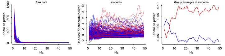
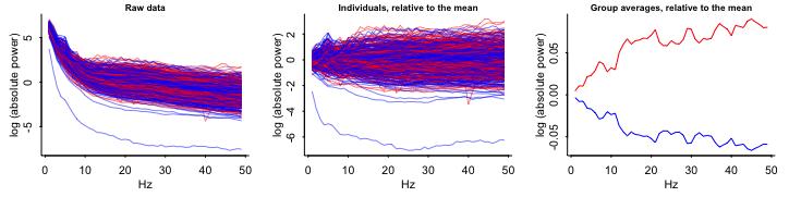
- Outcome:
- Top: Absolute EEG (brainwaves) power; X-axis is frequency
- Bottom Log Absolute EEG (brainwaves) power; X-axis is frequency
- Blue: Each control group patient
- Red: Each treatment group patient
- Outcome:
- Interpretations
- Raw, z-scores, Relative to mean:
- Not Logged: substantial overlap between Control and Treatment groups
- Logged: Control and Treatment groups almost completely overlap
- Group averages relative to the mean at each frequency:
- So grouped by group, frequency \(\rightarrow\)
mutate(mean)? - Substantial differences
- So grouped by group, frequency \(\rightarrow\)
- Raw, z-scores, Relative to mean:
- Compare sample data with random-chance data
Keep the same observations but randomly permute the treatment assignment variable and see what happens
Repeat (e.g. 9 times)
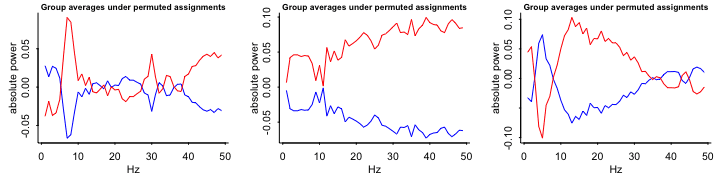
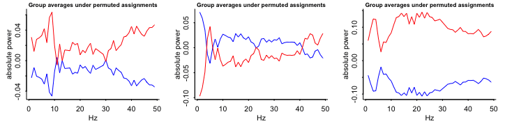
- Group averages: patterns in these random permutations don’t look so different, either qualitatively or quantitatively, from what we saw from the actual comparison
- The red line is on top most of the time and substantially separated from the blue line 3 out fo the 9 times.
- Group averages: patterns in these random permutations don’t look so different, either qualitatively or quantitatively, from what we saw from the actual comparison
- Variables
Log response if:
- All the measurements are positive
- Seems reasonable to start with proportional effect
Include pre-test brain activity as a predictor (baseline)
Fit
y ~ z + x- y: Outcome (Log Brain Activity)
- z: Treatment Indicator
- x: Pre-Treatment Measure
Try including interaction of x and z
Plot y vs. x with blue dots for the controls (z = 0) and red dots for the treated kids (z = 1).
- Example 3: Soloman, RCT, 2 groups, unequal treatment schedule
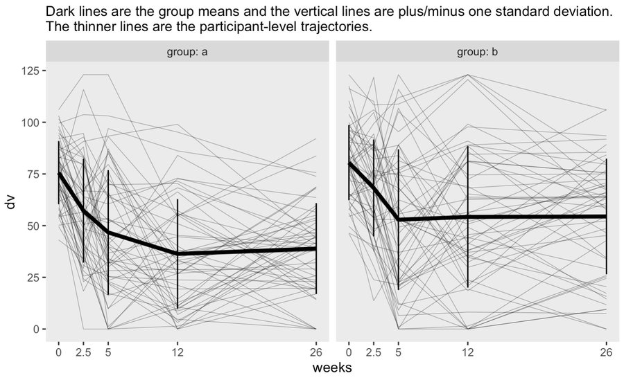
- Notes from: Thread
- First three time points are baseline, mid-treatment, and immediately post-treatment. The last two are follow-ups
- Nonlinear means indicate a GAM would be a good option
- Solution
- GAM:
mgcv::gam(data, y ~ 1 + group + s(weeks, by = group, k = 4) + s(week, subject, bs = "fs", k = 4))- A “random smooth” for subjects and not just a random intercept
- subject is a factor variable
- fs is a factor smooth spline
predict(fit, exclude = "s(weeks,subject)")- Computes the population fitted lines
gratia::smooths(model)will return the labels for all smooths in the model, so you know what you need for the exclude call without having to callsummary()
- GAM:
- Example 4: Randomized Complete Block Design (RCBD)
Data
head(dataset)
##   block density yield
## 1     1       0 29.90
## 2     2       0 34.23
## 3     3       0 37.12
## 4     4       0 26.37
## 5     5       0 34.48
## 6     6       0 33.70
Do not model with block as a fixed effect
mod.reg <- lm(yield ~ block + density, data = dataset)- Assumes that the blocks produce an effect only on the intercept of the regression line, while the slope is unaffected
Do model with block as a random effect (i.e. block effect may produce random fluctuations for both model parameters, intercept and slope)
library(nlme)

modMix.1 <-
  lme(yield ~ density,
      random = ~ density|block,
      data=dataset)

# or equivalently

modMix.1 <-
  lme(yield ~ density,
      random = list(block = pdSymm(~density)),
      data=dataset)
## Linear mixed-effects model fit by REML
##  Data: dataset
##        AIC      BIC    logLik
##  340.9166 355.0569 -164.4583
##
## Random effects:
##  Formula: ~density | block
##  Structure: General positive-definite, Log-Cholesky parametrization
##            StdDev    Corr
## (Intercept) 3.16871858 (Intr)
## density    0.02255249 0.09
## Residual    1.38891957
##
## Fixed effects: yield ~ density
##                Value Std.Error DF  t-value p-value
## (Intercept) 31.78987 1.0370844 69  30.65311      0
## density    -0.26744 0.0096629 69 -27.67704      0
##  Correlation:
##        (Intr)
## density -0.078
##
## Standardized Within-Group Residuals:
##        Min        Q1        Med        Q3        Max
## -1.9923722 -0.5657555 -0.1997103  0.4961675  2.6699060
##
## Number of Observations: 80
## Number of Groups: 10
If there is NOT a strong correlation between the slope (e.g. listed above as corr = 0.09 for density) and intercept (i.e. correlated random effects) in the Random Effects section of
summary(modMix.1), try modeling with the random effects as independentmodMix.2 <- lme(yield ~ density, random = list(block = pdDiag(~density)), data=dataset)pdDiagspecifies a var-covar diagonal matrix, where covariances (off-diagonal terms) are constrained to 0Check if the change made a significant difference (i.e. pval < 0.05)
anova(modMix.1, modMix.2)
Other options include: either random intercept or random slope
# Model with only random intercept
modMix.3 <-
  lme(yield ~ density,
      random = list(block = ~1),
      data=dataset)
# Alternative notation
# random = ~ 1|block

# Model with only random slope
modMix.4 <-
  lme(yield ~ density,
      random = list(block = ~ density - 1),
      data=dataset)
# Alternative notation
# random = ~density - 1 | block
Fitting a nonlinear model
library(aomisc)
datasetG <- groupedData(yieldLoss ~ 1|block, dataset)
nlin.mix <-
  nlme(yieldLoss ~ NLS.YL(density, i, A),
       data=datasetG,
       fixed = list(i ~ 1, A ~ 1),
       random = i + A ~ 1|block)

# or equivalently

nlin.mix2 <-
  nlme(yieldLoss ~ NLS.YL(density, i, A),
       data=datasetG,
       fixed = list(i ~ 1, A ~ 1),
       random = pdSymm(list(i ~ 1, A ~ 1)))

## Nonlinear mixed-effects model fit by maximum likelihood
##  Model: yieldLoss ~ NLS.YL(density, i, A)
##  Data: datasetG
##        AIC      BIC    logLik
##  474.8225 491.5475 -231.4113
##
## Random effects:
##  Formula: list(i ~ 1, A ~ 1)
##  Level: block
##  Structure: General positive-definite
##          StdDev    Corr
## i        0.1112839 i
## A        4.0466971 0.194
## Residual 1.4142009
##
## Fixed effects: list(i ~ 1, A ~ 1)
##      Value Std.Error  DF  t-value p-value
## i  1.23242  0.038225 104 32.24107      0
## A 68.52068  1.945173 104 35.22600      0
##  Correlation:
##  i
## A -0.409
##
## Standardized Within-Group Residuals:
##        Min        Q1        Med        Q3        Max
## -2.4414051 -0.7049356 -0.1805322  0.3385275  2.8787362
##
## Number of Observations: 120
## Number of Groups: 15
Exclude correlation between random effects (0.194 above) if not substantial for a simpler model
nlin.mix3 <-
  nlme(yieldLoss ~ NLS.YL(density, i, A),
       data = datasetG,
       fixed = list(i ~ 1, A ~ 1),
       random = pdDiag(list(i ~ 1, A ~ 1)))