Loss Functions
Misc
- Also see
- Packages
- {SLmetrics} (github)- Very fast, written in C++
- {yardstick} - {tidymodels}
- {MLmetrics}
- {mlr3measures} - {mlr3}
- Make sure your Loss Function and Performance metrics correlate
- Loss function are typically minimized and metrics are typically maximized. So, when choosing a loss function, you should choose one that negatively correlates with your metric.
- Simulate some data, fit a model that using various loss functions, and score them with your performance metric. Then, choose the loss function that correlates with your metric the best.
- Example: Cross-Entropy vs. Accuracy
.png)
- Image is from a video, disregard the solid gridlines (actuallly video screens)
- X-Axis is Accuracy.
- Shows how the low values of the loss function correlate well with the performance metric, Accuracy.
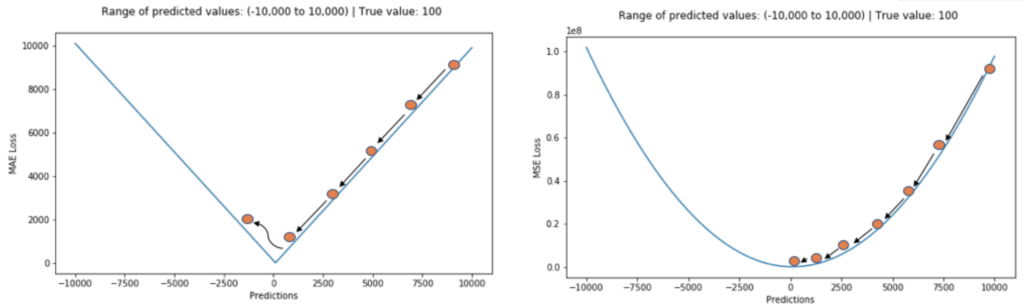
- Mean Absolute Error (MAE) isn’t typically used (instead of MSE) because it is not differentiable, thus gradient descent can’t be used to find its minimum. Stochastic Gradient Descent is used to overcome this problem. (See Algorithms, ML >> SVM >> Regression)
- When you optimize a model using the MAE or MSE, your model will end up predicting the median or mean of the distribution, respectively
- Absolute error is more robust to outliers
- Minimizes the median value whereas MSE minimizes the mean value
- Stochastic Gradient Descent: the gradient of the loss is estimated each sample at a time and the model is updated along the way with a decreasing strength schedule (aka learning rate)
- Also see Model building, sklearn >> Algorithms>> Stochaistic Gradient Descent (SGD)
0/1 Loss (aka binary loss)
\[\begin{align} &L_{0/1}(h) = \frac{1}{n} \sum_{i=1}^n \delta_{h(x_i) \ne y_i} \\ &\text{where} \;\; \delta_{h(x_i) \ne y_i} = \left\{ \begin{array}{lcl} 1, & \mbox{if} \; h(x_i) \ne y_i \\ 0, & \mbox{otherwise} \end{array}\right. \end{align}\]
- It’s basically the misclassification rate (additive inverse of accuracy) but as a loss function
- Sum the 1s for misclassified labels and 0 for correct classifications. Then, take the average
- 1 (or maybe 0 too) doesn’t have to be the incorrect classification value. You could weight the incorrect classifications differently. If it’s 2, then you’d double the weight against an incorrect classifcation. Although it wouldn’t be 0/1 loss anymore.
- Often used to evaluate classifiers, but is not useful in guiding optimization since it is non-differentiable and non-continuous.
Area Under the Minimum
- Short for Area Under Min(FP, FN)
- A loss function that optimizes for AUC in classification models
- Paper: Optimizing ROC Curves with a Sort-Based Surrogate Loss for Binary Classification and Changepoint Detection
- {torchMAUM} - Multi-Class Area Under the Minimum in Torch
Asymmetric Huber Loss
\[F_H(x) = \left\{\begin{array}{lcl} -\theta_L (2x + \theta_L) & \mbox{for} \; -\infty \lt x \lt -\theta_L \\ x^2 & \mbox{for} \; -\theta_L \le x \lt \theta_R \\ \theta_R(2x-\theta_R) & \mbox{for} \; \theta_R \le x \lt \infty \end{array}\right.\]
\(\theta\) is the \(\delta\) in Huber loss. There are two “delta” parameters now to adjust the amount of asymmetry on either the left/lower half (\(\theta_L\)) or right/upper half (\(\theta_R\))
\(x\) is “\(y-f(x)\)” in Huber loss
The bottom condition, \(\theta_R(2x - \theta_R)\) is equivalent to the bottom condition in Huber loss
The top condition is just the conjugate(?) of the bottom condition
The “1/2” isn’t present in the middle condition for some reason as it is for the top condition in Huber loss.
- Checked Wiki and 1/2 is present in Huber loss there. Guess you could add it.
Potentially a more programmer-friendly version
\[F_H(X) = x^2 - \max\{(x - \theta_R), 0\}^2 - \max\{(-x - \theta_L), 0\}\]
- Not sure about the x2 part
Average Relative Mean Squared Error
\[\begin{align} &\text{ARMSE}_j = \left(\prod_{i=1}^n \frac{\mbox{MSE}_{i,j}}{\mbox{MSE}_{i,b}} \right)^{\frac{1}{n}} \\ &\text{where} \;\; \mbox{MSE}_{i,j} = \frac{1}{QH} \sum_{q=1}^Q \sum_{h=1}^{H} (\bar y_{q,h,i,j} - y_{q,h,i})^2 \end{align}\]
- \(\bar y\) : Either the base forecast (\(\hat y\)) or the reconciled forecast (\(\tilde y\))
- \(Q\) : Index of the forecast origins (?, Paper was not clear about what this is)
- \(H_k\) : Forecast Horizon
- \(n\) : The number of individual time series
- \(j, b\) : The forecast model and the naive (or benchmark) model respectively
- A normalized measure of error that allows for a consistent assessment relative to the benchmark
- Source
Brier Loss
\[\text{Brier Loss} = (y_{\mbox{pred}} - y_{\mbox{true}})^2\]
- How far your predictions lie from the true values
- A mean square error in the probability space
Expectile Loss
\[\text{EL} = \frac{1}{N} \sum_{i=1}^N \left | \alpha - \mathbb{1}(f(x_i) - \hat f(x_i) \lt 0) \right | \cdot (f(x_i) - \hat f(x_i))^2\]
- Similar to how quantile loss minimizes MAE using a weighting scheme, expectile loss minimizes MSE using a weighting scheme.
- Since your essentially minimizing MSE, your model’s estimate will be more sensitive to larger errors.
- See Quantile Loss for details on the weighting scheme
- See Regression, Quantile for packages for Expectile Regression
- If you want to penalize underpredictions more heavily, you want to predict a higher “expectile” than the 50th expectile (aka mean).
- e.g. In estimating Value-at-Risk, you might use \(\alpha\) >> 0.50 to heavily penalize large unexpected losses (i.e. underpredictions) while still maintaining some sensitivity to gains
- Using the 50th expectile would be equivalent to using OLS regression.
Focal Loss
\[\text{FL}(p) = \left\{\begin{array}{lcl} -\alpha(1-p)^\gamma \; \log(p), & y = 1 \\ -(1-\alpha) \; p^\gamma \; \log(1-p), & \text{otherwise} \end{array}\right.\]
- Where \(\gamma\) is the focusing parameter and \(\alpha\) is a class balancing weight
- Both are hyperparameters that can be tuned during CV
- \(\gamma = 0\) results in the cross-entropy formula
- As \(\gamma\) gets larger, the more importance will be given to misclassified examples and less importance towards easy examples.
- \(\gamma = 2\) and \(\alpha =.25\) is a recommended starting points (paper)
- \(\alpha\) can be set as the inverse class frequency
- \(\gamma = 2\) and \(\alpha =.25\) is a recommended starting points (paper)
- Gist with Focal loss function for keras
- Focuses on the examples that the model gets wrong rather than the ones that it can confidently predict, ensuring that predictions on hard examples improve over time rather than becoming overly confident with easy ones
Geometric Trace Mean Squared Error (GTMSE)
\[\text{GTMSE} = \sum_{j=1}^h \log \frac{1}{T-j}\sum_{t=1}^{T-j} e^2_{t+j|t}\]
- Multi-step Estimators and Shrinkage Effect in Time Series Models
- Forecasting loss function that imposes shrinkage on parameters similar to other estimators but does it more mildly because of the logarithms in the formula
- What the logarithms do is make variances of all forecast errors similar to each other. As a result, when used, GTMSE does not focus on the larger variances as other methods do but minimizes all of them simultaneously similarly.
- Making models less stochastic and more inert. Therefore, performance depends on each specific situation and the available data and shouldn’t be used universally.
- Packages: {smooth}, {greybox}
Huber Loss
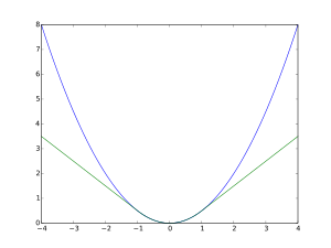
\[L_\delta (y, f(x)) = \left\{\begin{array}{lcl} \frac{1}{2} (y-f(x))^2, & \mbox{for} \; |y - f(x)| \lt \delta \\ \delta(|y-f(x)| - \frac{1}{2} \delta), & \text{otherwise} \end{array}\right.\]
- Huber loss (green, \(\delta =1\)) and squared error loss (blue) as a function of \(y-f(x)\)
- A combination of squared loss and absolute loss
- For residuals > \(\delta\), the absolute value of the residual is used which is based on the unbiased estimator of the median
- Therefore more robust to outliers
- The loss is the square of the usual residual (\(y - f(x)\)) only when the absolute value of the residual is smaller than a fixed parameter, \(\delta\).
- For residuals > \(\delta\), the absolute value of the residual is used which is based on the unbiased estimator of the median
- \(\delta\) is a tuneable parameter
- The function is quadratic for small values of \(|y - f(x)|\), and linear for large values
- Commonly used in deep learning where it helps to avoid the exploding gradient problem due to its insensitivity to large errors.
- {yardstick::huber_loss}
Mean Absolute Log Error (MALE)
\[\text{MALE} = \frac{1}{T} \sum_{t=1}^T \left|\log \left(\frac{f_t}{y_t}\right)\right|\]
- article
- \(f\) is the forecast and \(y\) is the observed
- Similar to RMSLE
- Requirement: data are strictly positive: they do not take zero or negative values
- Predicts the median of your distribution
- Underestimates and overestimates are punished equally harshly
- Transform it back onto a relative scale by taking the exponential (
exp(MALE)) which is the (geometric) mean relative error - Interpetation:
- Example:
exp(MALE)of 1.2 means you expect to be wrong by a factor of 1.2 in either direction, on average. (Explain this to your boss as a 20% average percentage error.)
- Example:
- Comparison with MAPE, sMAPE
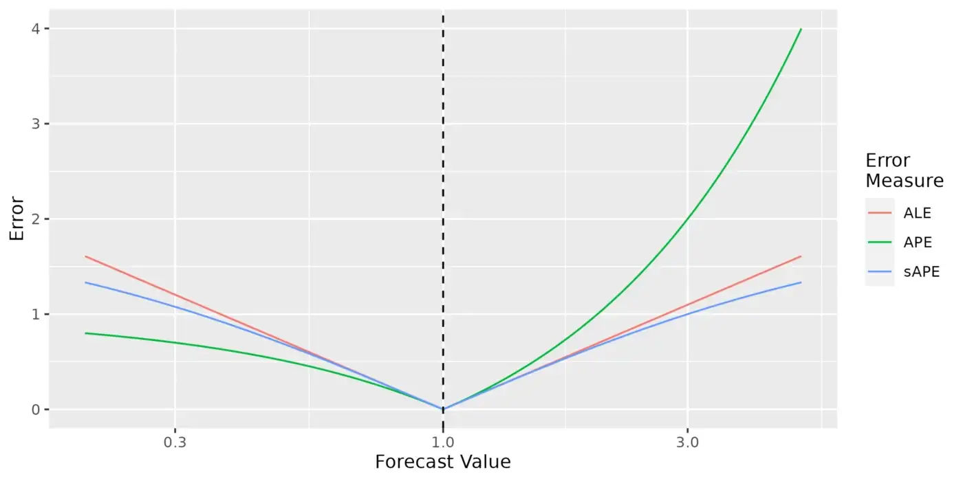
- Provided your errors are sufficiently small (e.g. less than 10%), it probably doesn’t make much difference which of the MALE, sMAPE or MAPE you use.
- MALE is is between the MAPE and sMAPE in sensitivity to outliers. For
- Example: Compared to being wrong by +10x, being wrong by +100x gives you 1.2 times your original sMAPE, 2 times your original MALE, and 9 times your original MAPE.
Mean Absolute Scaled Error (MASE)
\[\text{MASE} = \mbox{mean}(|q_j|)\]
Alternative to using percentage errors (e.g. MAPE) when comparing forecast accuracy across series with different units since it is independent of the scale of the data
Greater than 1: Worse than the average naive forecast
Less than 1: Better than the average naive forecast
Non-seasonal time series scaled error
\[q_j = \frac{e_j}{\frac{1}{T-1} \sum_{t=2}^T |y_t - y_{t-1}|}\]
Seasonal time series scaled error
\[q_j = \frac{e_j}{\frac{1}{T-1}\sum_{t = m+1}^T |y_t - y_{t-m}|}\]
Mean Absolute Scaled Log Error (MASLE)
\[\begin{align} \mbox{SLE}_{T+h} &= \frac{|\log\left(\frac{f_{T+h}}{y_{T+h}}\right)|}{\frac{1}{T-1}\sum_{t=2}^T |\log\left(\frac{y_{t-1}}{y_t}\right)|} \\ \text{MASLE} &= \mbox{mean}(\text{SLE}) \end{align}\]
- \(f\) is the forecast and \(y\) is the observed
- Scaled version of MALE
- It’s been normalized by the error of a benchmark method (e.g. the naive or seasonal naive methods) to place the errors on the same scale
Mean Balanced Log Loss (aka Balanced Cross-Entropy)
\[\text{BCE}(p, \hat p) = -\frac{1}{N} \sum_{i=1}^N (\beta \cdot p \log(\hat p) + (1-\beta)(1-p)\log(1-\hat p)) \]
- Adds a weight, \(\beta\), to the log loss formula to handle class imbalance
- Can tune during CV
- Where \(p\) is the observed 0/1 and \(\hat p\) is the predicted probability
- For just balanced log-loss, remove the summation and 1/N
Mean log loss (aka cross-entropy)
\[\text{CE} = -\frac{1}{N} \sum_{i=1}^N (y_i \cdot \log(p(y_i)) + (1-y_i) \cdot \log(1-p(y_i)))\]
- \(p(y_i)\) is the predicted probability and \(y_i\) is the observed 0/1
- For just log-loss, remove the summation and 1/N
- If the model predicts that an observation should be labeled 1 and assigns a high probability to that prediction, a high penalty will be incurred when the true label is 0. If the model had assigned a lower probability to that prediction, a lower penalty would have been incurred
- Might be equivalent to K-L Divergence
- Above equation is for a binary model but can be extended multiclassification models
- You’d replace the above expression and have a term for each category — each being \(y_i \cdot \log(p(y_i))\) where each \(p(y_i)\) is the probability for that category
- {yardstick::mn_log_loss}
- Notes
- Handles class imbalance poorly
- In sliced season 2 w/Silge on bird strike dataset, mean log loss scored a balanced outcome variable better than the unbalanced one.
- Fails to distinguish between hard and easy examples. Hard examples are those in which the model repeatedly makes huge errors, whereas easy examples are those which are easily classified. As a result, Cross-Entropy loss fails to pay more attention to hard examples.
- Handles class imbalance poorly
Mean Squared Error (MSE)
A quadratic loss function that’s calculation is based on the squared errors, so it is more sensitive to the larger deviations associated with tail events
A custom asymmetric MSE loss function can better account for large deviations in errors
\[\mbox{MSE}_{\text{cust}} = \frac{1}{n} \sum_{i=1}^n |\alpha - \mathbb{1}\{g(x_i) - \hat g(x_i) \lt 0\}| \cdot (g(x_i) - \hat g(x_i))^2\]
- With \(\alpha \in(0,1)\) being the parameter we can adjust to change the degree of asymmetry
Quantile Loss
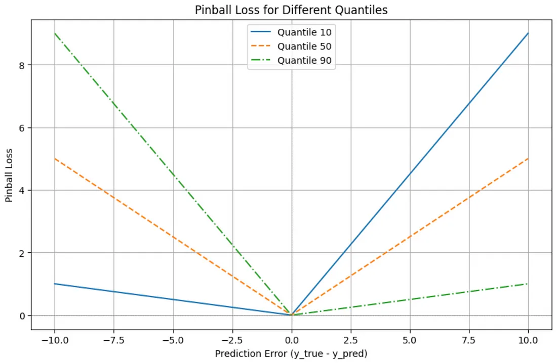
\[\frac{1}{n} \sum_{i=1}^n \left | \tau - \mathbb{1}(f(x_i) - \hat f(x_i) \lt 0) \right | \cdot \left | f(x_i) - \hat f(x_i) \right |\]
- AKA Pinball Loss
- \(\tau \in (0, 1)\) is the quantile. Residuals less than 0 use \(\tau - 1\) as a penalty and residuals greater than 0 use \(\tau\)
- Allows you to predict a certain percentile of the outcome variable
- Not effective at predicting tail events
- Using the median assigns equal weights to underpredictions and overpredictions. This is also equivalent to using the MAE loss function, i.e. Least Absolute Deviations (LAD) Regression.
- i.e. if we’re worried about underpredictions more, we should choose to predict a higher quantile than the median and vice versa if we’re worried more about overpredictions.
- For quantiles greater than 50, underpredictions are penalyzed more than overpredictions
- The asymmetrical penalty pushes the model to prefer overprediction to underprediction for high quantiles which places importance of accurately capturing higher values in the distribution
- Example: 90th quantile (source)
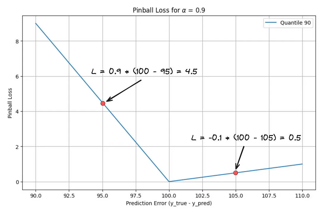
- X-Axis is mislabelled — it’s just the prediction value.
- 100 is the vertex which is the actual value and a prediction of 105 is a loss value of 0.5
- Underpredictions (when the actual value is greater than the predicted value): The penalty is 0.9 * (actual - predicted)
- Overpredictions (when the actual value is less than or equal to the predicted value): The penalty is -0.1 * (actual - predicted)
- The intuition behind this is that for the 90th quantile, we expect the actual value to be below our prediction 90% of the time. When it’s not (i.e., when we underpredict), we incur a much larger penalty.
- For quantiles less than 50, overpredictions are penalyzed more than underpredictions
- Similar reasoning.
Relative Absolute Error
\[\mbox{RAE} = \frac{\hat y - y}{y}\]
Root Mean Squared Logarithmic Error (RMSLE)
\[\text{RMSLE} = \sqrt{\frac{1}{n} \sum_{i=1}^n (\log(\hat y_i + 1) - \log(y_i + 1))^2}\]
Also see Understanding the metric: RMSLE
Mainly used when predictions have large deviations. Values range from 0 up to millions and we don’t want to punish deviations in prediction as much as with MSE
Predicts the geometric mean of your distribution
- The geometric mean is most useful when numbers in the series are not independent of each other or if numbers tend to make large fluctuations.
Similar to MALE except the
exp(RMSLE)is still not directly intepretableYou can just add 1 to your outcome then log it then used RMSE for your loss
Drob did
log(outcome) + 1but that doesn’t match the formula so I dunno if he’s right.mutate(outcome = log(outcome + 1)
{SLmetrics::rmsle or weighted.rmsle}
- Weighted case for heteroskedastic residuals
Extend {yardstick} by creating a custom metric to calculate RMSLE
library(rlang)
rmsle_vec <- function(truth, estimate, na_rm = TRUE, ...) {
  rmsle_impl <- function(truth, estimate) {
    sqrt(mean((log(truth + 1) - log(estimate + 1))^2))
  }
  metric_vec_template(
    metric_impl = rmsle_impl,
    truth = truth,
    estimate = estimate,
    na_rm = na_rm,
    cls = "numeric",
    ...
  )
}
rmsle <- function(data, ...) {
  UseMethod("rmsle")
}
rmsle <- new_numeric_metric(rmsle, direction = "minimize")
rmsle.data.frame <- function(data, truth, estimate, na_rm = TRUE, ...) {
  metric_summarizer(
    metric_nm = "rmsle",
    metric_fn = rmsle_vec,
    data = data,
    truth = !!enquo(truth),
    estimate = !!enquo(estimate),
    na_rm = na_rm,
    ...
  )
}
Root Mean Squared Scaled Error (RMSSE)
\[\begin{align} &\text{RMSSE} = \frac{1}{\sqrt{\frac{1}{T-1}\sum_{t=1}^{T-1} \Delta^2_t}}\text{RMSE} \\ &\text{where}\;\; \text{RMSE} = \sqrt{\frac{1}{h}\sum_{j=1}^h e^2_{t+j}} \end{align}\]
- \(\Delta_t\) is the first differences of the in-sample values
- Used in the M5 Competition
- {greybox::RMSSE}
Scaled Absolute Mean Error (SAME)
\[\begin{align} &\mathrm{SAME} = \frac{1}{\frac{1}{T-1} \sum_{t=1}^{T-1} |\Delta_t|} \mathrm{AME} \\ &\text{where}\;\;\mathrm{AME}= \left| \frac{1}{h} \sum_{j=1}^h e_{t+j} \right| \end{align}\]
- \(\Delta_t\) is the first differences of the in-sample values
- Similar to MASE, but measures bias
- {greybox::SAME}
Symmetric Mean Absolute Percentage Error (SMAPE)
\[\text{SMAPE} = \frac{100}{n} \sum_{i=1}^n \frac{|\hat y - y|}{\frac{1}{2}(|\hat y| + |y|)}\]
Code
smape <- function(a, f) {return (1/length(a) * sum(2*abs(f-a) / (abs(a)+abs(f))*100))}Packages: {yardstick}, {Metrics}
Check notebook — think this metric has issues with values around 0
Handles data where the scale varies over time; it is relatively comparable across time series; deals reasonably well with outliers
Underestimates and overestimates are punished equally harshly
- MAPE punished overestimates more severely than underestimates
Weighted Root Mean Square Scaled Error (WRMSSE)
\[\begin{align} &\text{RMSSE} = \frac{\sqrt{\frac{1}{h}\sum_{t=1}^h(\hat y_t - y_t)^2}}{\sqrt{\frac{1}{n-1}\sum_{t=2}^n (y_t-y_{t-1})^2}} \\ &\text{WRMSSE} = \sum_{p \in P} w_p \times \text{RMSSE}_p \end{align}\]
- Notes from Sales Forecasts – Part 1. Evaluation
- RMSSE is the scaled RMSE and is for a single forecast. It’s scaled by the RMSE of the naive forecast (denominator)
- WRMSSE seems to be for maybe a multivariate forecast or grouped/global forecast.
- \(n\) is the number of observations in your training data
- \(w_p\) is the weight for category \(p\) (e.g. product, store, etc.)
- The weight is on an error, so I’m guessing it’s a sort of cost with more weight going to the more important unit category. “Importance” maybe is determined by the cost of losing a sale of the item or the cost of storing an item.