Clustering
Misc
- Also see Notebook, pg 57
- Packages
- {clusterv} - Assessment of Cluster Stability by Randomized Projections
- {clusterindices} - Numerous indices to choose the optimal number of clusters when performing k-means.
- {DBCVindex} - Calculates the Density-Based Clustering Validation (DBCV) Index
- {fpc} - Cluster validation statistics for distance based clustering including corrected Rand index. Standardisation of cluster validation statistics by random clusterings and comparison between many clustering methods and numbers of clusters based on this. Cluster-wise cluster stability assessment.
- Methods for estimation of the number of clusters: Calinski-Harabasz, Tibshirani and Walther’s prediction strength, Fang and Wang’s bootstrap stability. Gaussian/multinomial mixture fitting for mixed continuous/categorical variables.
- Variable-wise statistics for cluster interpretation
- {genieclust} - Internal Cluster Validity Measures. Provided index functions set up so that the greater the output value (index), the more “valid” the clustering
- Metrics: Calinski Harabasz, Dunnowa, Generalized Dunn, Ball Hall, Davies Bouldin, WCSS, Silhouette, and Silhouette W
- See Are cluster validity measures (in)valid? for an overview of the indicies
- {GOFclustering} - Goodness-of-Fit Testing for Model-Based Clustering. Implements a test statistic derived from empirical likelihood to verify the distribution of clusters in multivariate Gaussian mixtures and other latent class models.
- {mosclust} - Assesses clustering by perturbation of the data and measuring the stability of clustering. (i.e. if the same clusters are produced, it’s a good model). Created with biological data in mind, but I think it should work elsewhere.
- Assessment of the reliability of a given clustering solution
- Finds if there is “natural” number of clusters
- Assessment of the statistical significance of a given clustering solution
- Tests if there are multiple reliable clustering solutions at a given significance level
- {Silhouette} - Proximity Measure Based Diagnostics for Standard, Soft, and Multi-Way Clustering
- Quantifies clustering quality by measuring both cohesion within clusters and separation between clusters
- Implements advanced silhouette width computations for diverse clustering structures, including: simplified silhouette
- For K-Means, elbow method (i.e. WSS) is awful. Recommended: Calinski-Harabasz Index and BIC then either Silhouette Coefficient or Davies-Bouldin Index
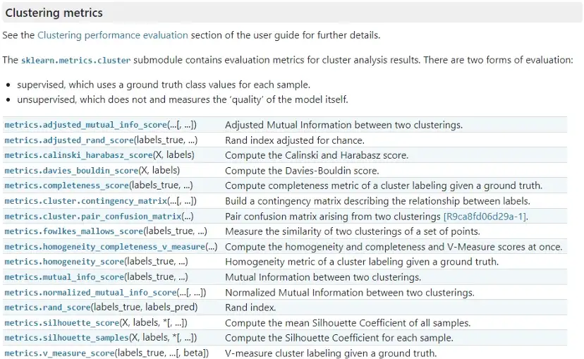
- {sklearn.metrics.cluster}
Cluster Validity Indices (CVI)
- Notes from {dtwclust} vignette
- Types
- For either Hard (aka Crisp) or Soft (aka Fuzzy) Partitioning
- Internal (IVI) - Tries to define a measure of cluster purity
- External (EVI) - Compares the obtained partition to the correct one. Thus, external CVIs can only be used if the ground truth is known
- Issues
- Associated, ground truth class labels do not necessarily correspond to recoverable, natural clusters
- High EVI scores reliably indicate good label recovery, low EVI scores do not necessarily indicate poor clustering structure in a partition, given the possibility of legitimate alternatives
- These concerns can be mitigated by instead utilizing datasets where cluster labels have been curated to encompass those formal and informal cluster concepts deemed important for the problem and domain according to the relevant experts.
- Manually labelling such datasets can be tedious and expensive. Synthetic datasets where the generation process is informed by the literature and expert opinion is a more efficient alternative.
- Issues
- Relative (RVI) - Attempt to quantify the extent to which a partition exemplifies one or more generally desirable cluster concepts, such as small within-group dissimilarities, large between group dissimilarities or effective representation by cluster prototypes
- e.g. Silhouette Width Criterion and Davies-Bouldin Index
- Issues (source)
- Comparisons based on RVIs will be biased towards those partitions and methods that align with the primarily domain-agnostic cluster concepts inherently preferred by different RVIs
- RVIs show a tendency to insufficiently penalize large, noisy clusters, and favor partitions that isolate outliers
- The use of RVIs for any comparisons of normalization procedures, representation methods and distance measures are highly dubious due to the influence of these components on pairwise dissimilarities
- Scores
.png)
- Available through
dtwclust::cvi - Global centroid is one that’s computed using the whole dataset
- dtwclust implements whichever distance method that originally used in the clustering computation
- Some CVIs require symmetric distance functions (distance from a to b = distance b to a)
- A warning is printed if an asymmetric distance method was used
- {clue} - Compare repetitions of non-deterministic clustering methods (e.g. partitional) where random element means you get a different result each time
- It uses a measure called “dissimilarities using minimal Euclidean membership distance” to compare different runs of a cluster method
- Available through
Spherical/Centroid Based
- Within-Cluster Sum of Squares (WSS) (aka Inertia)
- Measures the variability of the observations within each cluster. In general, a cluster that has a small sum of squares is more compact than a cluster that has a large sum of squares.
- To calculate WCSS, you first find the Euclidean distance between a given point and the centroid to which it is assigned. You then iterate this process for all points in the cluster, and then sum the values for the cluster and divide by the number of points
- Influenced by the number of observations. As the number of observations increases, the sum of squares becomes larger. Therefore, the within-cluster sum of squares is often not directly comparable across clusters with different numbers of observations.
- To compare the within-cluster variability of different clusters, use the average distance from centroid instead.
- Typically used in the elbow method for kmeans for choosing the number of clusters
- Average Distance from Centroid
- The average of the distances from observations to the centroid of each cluster.
- The average distance from observations to the cluster centroid is a measure of the variability of the observations within each cluster. In general, a cluster that has a smaller average distance is more compact than a cluster that has a larger average distance. Clusters that have higher values exhibit greater variability of the observations within the cluster.
- Silhouette Coefficient
Computationally expensive
Formula
\[s(i) = \frac{b(i) - a(i)}{\max \{a(i), b(i)\}},\; \text{if}\; |C_I| > 1\]
Intra-Cluster Distance
\[a(i) = \frac{1}{|C_I| - 1} \sum_{j \in C_I, i \neq j} d(i,j)\]
- The mean distance between i and all the other data points within C.
- \(|C_I|\) is the number of points belonging to cluster i, and d(i , j) is the distance between data points i and j in the cluster CI
Inter-Cluster Distance
\[b(i) = \min_{J \neq I} \frac{1}{C_J} \sum_{j \in C_J} d(i, j)\]
- The mean distance between i to all the points of its nearest neighbor cluster
Range: -1 to 1
Good: 1
Bad: -1
- Says inter-cluster distances are not comparable to the intra-cluster distances
- Calinski-Harabasz Index (aka Variance Ratio Criterion)
- {kpc::calinhara}:
calinhara(data, kmeans_results$cluster)orcluster.stats(data, kmeans_results$cluster)$chCompares the variance between-clusters to the variance within each cluster
NOT to be used to the density based methods, such as mean-shift clustering, DBSCAN, OPTICS, etc.
- Clusters in density based methods are unlikely to be spherical and therefore centroids-based distances will not be that informative to tell the quality of the clustering algorithm
- Much faster than Silhouette score calculation
Ratio of the squared inter-cluster distance sum and the squared intra-cluster distance sum for all clusters
Formula
\[CH = \frac{\sum_{k=1}^K n_k \lVert c_k - c \rVert^2}{K-1} \cdot \frac{N-K}{\sum_{k=1}^K \sum_{i=1}^{n_k} \lVert d_i - c_k \rVert^2}\]
- \(n_k\) is the size of the kth cluster
- \(c_k\) is the feature vector of the centroid of the kth cluster
- \(c\) is the feature vector of the global centroid of the entire dataset
- \(d_i\) is the feature vector of data point i
- \(N\) is the total number of data points
Range: no upper bound
Higher is better and means the clusters are separated from each other
- Davies-Bouldin Index
Average similarity between each cluster and its most similar one.
NOT to be used to the density based methods, such as mean-shift clustering, DBSCAN, OPTICS, etc.
- Clusters in density based methods are unlikely to be spherical and therefore centroids-based distances will not be that informative to tell the quality of the clustering algorithm
Much faster than Silhouette score calculation
Range [0,1] and lower is better
The type of norm used in the formula should probably match the distance type used in the clustering algorithm. See the wiki for details.
Formula
\[DB = \frac{1}{N} \sum_{i=1}^N D_i\]
An averaged similarity score across all clusters with its nearest neighbor cluster
\(D_i\) is the ith cluster’s worst (i.e. largest) similarity score, \(R_{i,j}\) across all other clusters
\[D_i = \max_{j\neq i} R_{i,j}\]
Smaller similarity score indicates a better cluster separation
\[\begin{aligned} &R_{i,j} = \frac{S_i + S_j}{M_{i,j}}\\ &\begin{aligned} \text{where} \;\; &S_i = \left(\frac{1}{T_i} \sum_{j=1}^{T_i} \lVert X_j - A_i \rVert_{p}^q \right)^{\frac{1}{q}} \;\; \text{and} \\ &M_{i,j} = \lVert A_i - A_j \rVert_p = \left(\sum_{k=1}^n |a_{k,i} - a_{k,j}|^p\right)^{\frac{1}{p}} \end{aligned} \end{aligned}\]
- \(X_j\) : n-dimensional feature vector assigned to Cluster \(C_i\)
- \(T_i\): The size of cluster \(C_i\)
- \(A_i\): Centroid of \(C_i\) and \(a_{k,i}\) is an element of the kth feature vector of \(A_i\) which has \(n\) elements
- \(P\): the degree of the norm; typically 2 for the euclidean norm (i.e. distance)
- \(q\): Not sure what this is (something to do with a statistical moment), but wiki only describes the parameter when it’s equal to 1 which makes S the average distance between the feature vectors and the centroid. So that’s probably the typical value.
Feature Reduction
- Bayesian Information Criteria (BIC)
Higher is better
GoF metric in this situation that’s typically used for GMMs
Not on the same scale as WSS
Py Code
def bic_score(X, labels):
  """
  BIC score for the goodness of fit of clusters.
  This Python function is directly translated from the GoLang code made by the author of the paper.
  The original code is available here: https://github.com/bobhancock/goxmeans/blob/a78e909e374c6f97ddd04a239658c7c5b7365e5c/km.go#L778
  """

  n_points = len(labels)
  n_clusters = len(set(labels))
  n_dimensions = X.shape[1]
  n_parameters = (n_clusters - 1) + (n_dimensions * n_clusters) + 1
  loglikelihood = 0
  for label_name in set(labels):
    X_cluster = X[labels == label_name]
    n_points_cluster = len(X_cluster)
    centroid = np.mean(X_cluster, axis=0)
    variance = np.sum((X_cluster - centroid) ** 2) / (len(X_cluster) - 1)
    loglikelihood += \
      n_points_cluster * np.log(n_points_cluster) \
      - n_points_cluster * np.log(n_points) \
      - n_points_cluster * n_dimensions / 2 * np.log(2 * math.pi * variance) \
      - (n_points_cluster - 1) / 2

  bic = loglikelihood - (n_parameters / 2) * np.log(n_points)

  return bic