Classification
Misc
- Also see Regression, Logistic
- Guide for suitable baseline models: link
- If you have mislabelled target classes, try AdaSampling to correct the labels (article)
Diagnostics
- Also see
- Diagnostics, Classification
- Regression, Logistic >> Diagnostics
- “During the initial phase of model building, a good strategy for data sets with two classes is to focus on the AUC statistics from these curves instead of metrics based on hard class predictions. Once a reasonable model is found, the ROC or precision-recall curves can be carefully examined to find a reasonable cutoff for the data and then qualitative prediction metrics can be used.” – 3.2.2 Classification Metrics” Kuhn and Kjell
- “Stable” AUC requirements for 0/1 outcome:
- Paper: Modern modelling techniques are data hungry: a simulation study for predicting dichotomous endpoints | BMC Medical Research Methodology | Full Text
- Logistic Regression: 20 to 50 events per predictor variable
- Random Forest and SVM: greater than 200 to 500 events per predictor variable
Class Imbalance
Misc
- Also see
- Model Building, tidymodel >> Recipe >> up/down-sampling
- Model Building, sklearn >> Preprocessing >> Class Imbalance
- Surveys, Analysis >> Modeling >> Tidymodels >> Importance weights
- Packages
- {themis} - Extra steps for the {recipes} for dealing with unbalanced data.
- {ebmc} - Four ensemble-based methods (SMOTEBoost, RUSBoost, UnderBagging, and SMOTEBagging) for class imbalance problem are implemented for binary classification.
- {imbalance} - Novel oversampling algorithms, filtering of instances and evaluation of synthetic instances. Methods: MWMOTE (Majority Weighted Minority Oversampling Technique), RACOG (Rapidly Converging Gibbs), wRACOG (wrapper-based RACOG), RWO (Random Walk Oversampling), and PDFOS (Probability Distribution density Function estimation based Oversampling).
- {imbalanced-learn} - Tools when dealing with {sklearn} classification with imbalanced classes
- {randomForestSRC} - Fast Unified Random Forests for Survival, Regression, and Classification (RF-SRC)
- Class Imbalanced q-classification
- Balanced random forests undersampling of the majority class. Performance is assesssed using the G-mean, but misclassification error can be requested.
- {ROBOSRMSMOTE} - Provides the ROBOSRMSMOTE (Robust Oversampling with RM-SMOTE) framework for imbalanced classification tasks
- Extends Mahalanobis distance-based oversampling techniques by integrating robust covariance estimators to better handle outliers and complex data distributions
- Applying SMOTE without re-calibration is bad (See van Smeden paper, thread)
- Or maybe just bad in general (StackExchange)
- Papers
- The harm of class imbalance corrections for risk prediction models: illustration and simulation using logistic regression
- Unless recalibration is applied, applying subsampling to correct class imbalance will lead to overpredicting the minority class (discrimination) and worse calibration when using logistic regression or ridge regression
- Paper used random undersampling (RUS), random oversampling (ROS), and SMOTE (Synthetic Minority Oversampling Technique)
- Event Fractions: 1%, 10%, 30%
- N: 2500, 5000; p: 3, 6, 12, 24
- “We anticipate that risk miscalibration will remain present regardless of type of model or imbalance correction technique, unless the models are recalibrated. However, class imbalance correction followed by recalibration is only worth the effort if imbalance correction leads to better discrimination of the resulting models.”
- They used what looked to be Platt Scaling for recalibration
- Also see Model Building, tidymodels >> Tune >> Tune Model with Multiple Recipes for an example of how downsampling (w/o calibration) + glmnet affects class prediction and GOF metrics
- The harm of class imbalance corrections for risk prediction models: illustration and simulation using logistic regression
- Subsampling can refer to up/oversampling or down/undersampling.
- It is perfectly ok to train a model on 1M negatives and 10K positives (i.e. plenty of events), as long as you avoid using accuracy as a metric
- 1K to 10K events might be enough for the ML algorithm to learn from
- For deep learning
- Loss Functions: Focal Loss and Label Smoothing.
- Optimization: Sharpness-Aware Minimization (SAM)
- A 50/50 balance is probably not optimal. (source)
- One paper that tested 20 datasets found that around 43% (number of minority events / number of majority events) was optimal.
- Other papers have found datasets where the optimal balance was over 50%
- Some categories can be more informative (i.e. easier to predict than others), so fewer events are necessary
- Best practice is treat the balance ratio as a hyperparameter and test a range of ratios as part of tuning.
- One paper that tested 20 datasets found that around 43% (number of minority events / number of majority events) was optimal.
- Also see
Issues
- Using Accuracy as a metric
- If the positivity rate is just 1%, then a naive classifier labeling everything as negative has 99% accuracy by definition
- If you’ve used subsampling, then the training data is not the same as the data used in production
- Low event rate
- If you only have 10 to 100 positive samples, the model may easily memorize these samples, leading to an overfit model that generalized poorly
- May result in large CIs for your effect estimate (see Gelman post)
- A potential disadvantage of upsampling is that new data is being created that could cause overfitting. Additionally, by artificially increasing the sample size standard errors will also be artificially decreased.
- A disadvantage of downsampling is that some data, and sometimes a lot of data, is excluded from the model.
- Using Accuracy as a metric
Check Imbalance
data %>%
  count(class) %>%
  mutate(prop = n / sum(n)) %>%
  pretty_print()
Downsampling/Undersampling
- Use cases for downsampling the majority class
- when the training data doesn’t fit into memory (and your ML training pipeline requires it to be in memory), or
- when model training takes unreasonably long (days to weeks), causing too long iteration cycles, and preventing you from iterating quickly.
- Using a domain knowledge filter for downsampling
- a simple heuristic rule that cuts down most of the majority class, while keeping nearly all of the minority class.
- e.g. if a rule can retain 99% of positives but only 1% of the negatives, this would make a great domain filter
- Examples
- credit card fraud prediction: filter for new credit cards, i.e. those without a purchase history.
- spam detection: filter for Emails from addresses that haven’t been seen before.
- e-commerce product classification: filter for products that contain a certain keyword, or combination of keywords.
- ads conversion prediction: filter for a certain demographic segment of the user population.
- a simple heuristic rule that cuts down most of the majority class, while keeping nearly all of the minority class.
- Use cases for downsampling the majority class
Hybrid
- Often done by oversampling the minority class and undersampling the majority class, and as before this could be done in a random fashion.
- Alternative: Removing some observations from both classes that would be nearest neighbors (TOMEK links)
- This should improve the model’s ability to classify the observations among those that remain, as they are more clearly delineated among the features.
Weighting
- Logistic Regression
- Weighting would essentially be equivalent to what is done with simple resampling techniques, negating the need to employ the latter.
- e.g. doubling the weight of an observation would be equivalent to having two copies of the observation in the dataset.
- Tree-based Models
- Weighting and resampling are not equivalent.
- e.g. in a random forest, resampling changes the composition of the bootstrap samples used to build the trees, while weighting changes the importance of each observation in the calculation of splits within each tree.
- Logistic Regression
CV
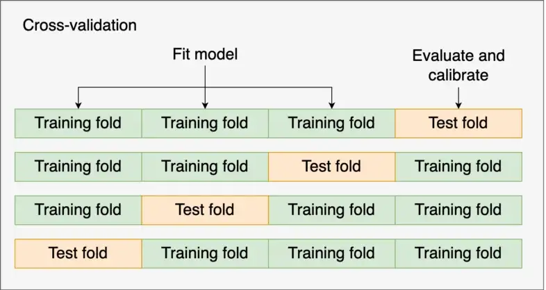
- It is extremely important that subsampling occurs inside of resampling. Otherwise, the resampling process can produce poor estimates of model performance.
- Data Leakage: if you first upsample the data and then split the data into training (aka analysis set) and validation (aka assessment set) folds, your model can simply memorize the positives from the training data and achieve artificially strong performance on the validation data, causing you to think that the model is much better than it actually is.
- The subsampling process should only be applied to the analysis (aka training) set. The assessment (aka validation) set should reflect the event rates seen “in the wild.”
- Does {recipe} handle this correctly?
- Process
- Subsample the data only in the analysis set
- Perform CV algorithm selection and tuning using a suitable metric for class imbalance
- Use same metric to get score on the test set
- It is extremely important that subsampling occurs inside of resampling. Otherwise, the resampling process can produce poor estimates of model performance.
ML Methods
- Synthetic Data Approaches
- TabDDPM: Modeling Tabular Data with Diffusion Models (Raschka Thread)
- Categorical and Binary Features: adds uniform noise via multinomial diffusion
- Numerical Features: adds Gaussian noise using Gaussian diffusion
- Synthetic Data Vault (Docs)
- Data generated with variational autoencoders adapted for tabular data (TVAE) (paper)
- Can Synthetic Data Boost Machine Learning Performance?
- TabDDPM: Modeling Tabular Data with Diffusion Models (Raschka Thread)
- Imbalanced Classification via Layered Learning (ICLL)
- For code, see article
- A hierarchical model composed of two levels:
- Level 1: A model is built to split easy-to-predict instances from difficult-to-predict ones.
- The goal is to predict if an input instance belongs to a cluster with at least one observation from the minority class.
- Level 2: We discard the easy-to-predict cases. Then, we build a model to solve the original classification task with the remaining data.
- The first level affects the second one by removing easy-to-predict instances from the training set.
- Level 1: A model is built to split easy-to-predict instances from difficult-to-predict ones.
- In both levels, the imbalanced problem is reduced, which makes the modeling task simpler.
- Synthetic Data Approaches
Tuning parameters
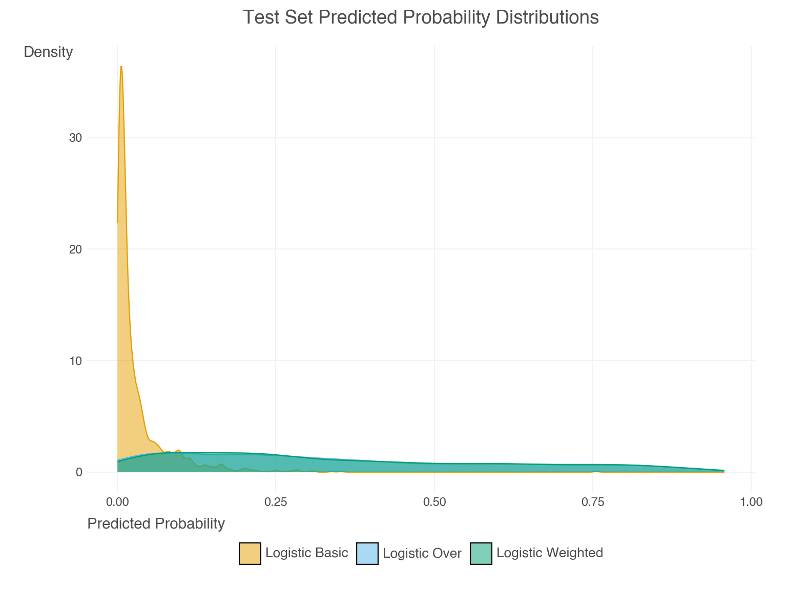
- Weighting and resampling often lead to over-prediction of the minority class. This can seen by examining the predicted probabilities directly. Their mean prediction is well beyond the observed rate
- XGBoost and LightGBM have a parameter called
scale_pos_weight, which up-weighs positive samples when computing the gradient at each boosting iteration - Unlikely to have a major effect and probably won’t generalize well.
- In Python,
- is_unbalance=True in {LightGBM}
- class_weight=‘balanced’ for logistic regression in {sklearn}
- Weighting and resampling often lead to over-prediction of the minority class. This can seen by examining the predicted probabilities directly. Their mean prediction is well beyond the observed rate
Calibration
- Calibrated- When the predicted probabilities from a model match the observed distribution of probabilities for each class. Sometimes described as the reliability of a model’s confidence in its predictions.
- Intuitively, if a model assigns a class with 90% probability, that class should appear 90% of the time.
- Calibration Plots visualize this comparison of distributions
- Calibration mesasure are important for validating a predictive model.
- Logistic Regression models are usually well-calibrated, but most ML and DL model predicted probabilities aren’t directly produced by the algorithms and aren’t usually calibrated
- RF models can also benefit from calibration although given enough data, they are already pretty well calibrated
- SVM, Naive Bayes, boosted tree algorithms, and DL models benefit most from calibration
- An unintended consequence of applying calibration can be the worsening of calibration for models that are already well calibrated
- If a model isn’t calibrated, then the magnitude of the predicted probability cannot be interpreted as the likelihood of an event
- e.g. If 0.66 and 0.67 are two predicted probabilities from an uncalibrated xgboost model, the 0.67 prediction cannot be interpreted as more likely to be an event than the 0.66 prediction.
- Miscalibrated predictions don’t allow you to have more confidence in a label with a higher probability than a label with a lower probability.
- Well-Ranked models (i.e. high AUC), where predicting target categories and not interpreting probabilities (e.g. risk) is the primary goal, will benefit less from calibration. Therefore, the extra resources required for calibration may not worth the effort.
- See (below) the introduction in the paper, “A tutorial on calibration measurements …” for examples of scenarios where calibration of risk scoring model is essential. If you can’t trust the predicted probabilities (i.e. risk) then decision-making is impossible.
- Also this paper which also explains some sources of miscalibration (e.g. dataset from region with low incidence, measurement error, etc.)
- Even if a model isn’t caibrated and depending on the metric, it can still be more accurate than a calibrated model.
- Poor calibration may make an algorithm less clinically useful than a competitor algorithm that has a lower AUC but is well calibrated (Calibration: the Achilles heel of predictive analytics)
- Calibration doesn’t affect the AUROC (does not rely on predicted probabilities) but does affect the Brier Score (does rely on predicted probabilities) (A tutorial on calibration measurements and calibration models for clinical prediction models)(Harrell)
- Since thresholds are based on probabilities, I don’t see how a valid, optimized threshold can be established for an uncalibrated model
- Wonder how this affects model-agnostic metrics, feature importance, shap, etc.
Misc
- Also see
- Diagnostics, Classification >> Calibration
- Econometrics, Propensity Score Analysis >> Misc >> Papers >> Calibration Strategies for Robust Causal Estimation: Theoretical and Empirical Insights on Propensity Score Based Estimators
- Provides insights on the calibration of RF and boosted tree models (used for propensity score creation) along with results from various CV calibration procedures. Includes code.
- Packages
- {probably} - tidymodels calibration package
- Calibration functions used in {tailor}. This package should be used for diagnostics of calibrated/non-calibrated probabilites
- Beta, Isotonic, Bootstrap Isotonic, Logistic, Multinomial, Linear (for regression models)
- Visualizing utilities and its evaluation metric is the average of the Brier scores (or anything in {yardstick}
- Calibrating Binary Probabilities - Nice tutorial
- {tailor} - Postprocessing of predictions for tidymodels;
- Creates an object class for performing calibration that can be set used with workflow objects, tuning, etc. Diagnostics of calibration seems to remain in {probably}.
- {{venn_abers}} (article) - Binary and Multi-Class Venn-ABERS calibration
- {rfUtilities::probability.calibration} - Isotonic Regression
- {platt} - Platt Scaling
- {MiMIR::plattCalibration} - Genomics package with a Platt Scaling function
- {betacal} - Beta Calibration
- {calibtools} - Posterior probability calibration methods for machine learning algorithms in R. It provides calibration
- Methods: isotonic regression, knn-based methods, Bayesian Binning into Quantiles (BBQ), Ensemble of Linear Trend Estimation (ELiTe) in multiclass case.
- Utilities for calibration performance measures and reliability diagrams.
- {CalibratR} - BBQ (Bayes Binning in Quantiles) model
- {{SelfCalibratingConformal}} (Paper) - Combines Venn-Abers calibration and conformal prediction to deliver calibrated point predictions alongside prediction intervals with finite-sample validity conditional on these predictions.
- {probably} - tidymodels calibration package
- Notes from:
- How and When to Use a Calibrated Classification Model with scikit-learn
- Can I Trust My Model’s Probabilities? A Deep Dive into Probability Calibration
- Python, multiclass example
- A tutorial on calibration measurements and calibration models for clinical prediction models (paper)
- Calibration curves for nested cv (post)
- For calibrated models, sample size affects the how well they’re calibrated
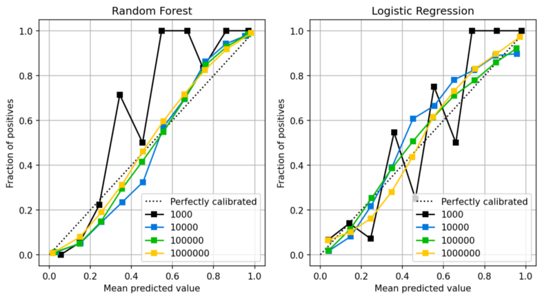
- Even for a logistic model, N > 1000 is desired for good calibration
- For a rf, closer to N = 10,000 is probably needed.
- Distributions of predicted probabilities
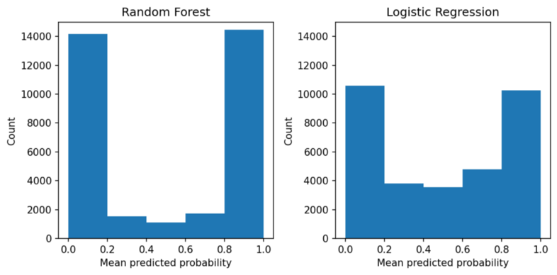
- Random Forest pushes the probabilities towards 0.0 and 1.0, while the probabilities from the logistic regression are less skewed.
- Decision Trees are even more skewed than RF
- Says how rare a prediction is.
- In a rf, really low or high probability predictions aren’t rare. So, if the model gives you a 0.93, you shouldn’t interpet it the way you normally would such a high probability (i.e. high certainty), because a rf inherently pushes its probabilities towards 0 and 1.
- Deep Learning Models
- Notes fromCalibration in Deep Learning: A Survey of the State-of-the-Art
- While increasing the depth and width of neural networks helps to obtain highly predictive power, it also negatively increases calibration errors. Empirical evidence has shown that this poor calibration is linked to overfitting on the negative log-likelihood (NLL).
- Some methods has been proposed to mitigate the impact of data noise on model calibration such as robust loss functions or adversarial training, have shown promise in improving model robustness to noisy data (Hendrycks, Mazeika, & Dietterich, 2018; Delaney, Greene, & Keane, 2021). Also Ensemble methods have been proofed effective in identifying and mitigating the effects of noisy data on model performance (Lakshminarayanan, Pritzel, & Blundell, 2017; Malinin, Mlodozeniec, & Gales, 2019).
- Techniques such as data augmentation (Muller et al., 2019; Zhang, Cisse, Dauphin, & Lopez-Paz, 2018), bias mitigation algorithms (Kamiran & Calders, 2012), and fairness-aware model training (Zemel, Wu, Swersky, Pitassi, & Dwork, 2013) can help mitigate biases during the model development stage.
Basic Workflow
- Misc
- Ideally you’d want each model (i.e. tuning parameter combination) being scored in a CV or a nested CV to have its own calibration model, but it’s not practical. But also, it’s unlikely an algorithm with a slightly different parameter value combination with have a substantially different predicted probability distribution, and it’s the algorithm itself that’s the salient factor. Therefore, for now, I’d go with 1 calibration model per algorithm.
- Process
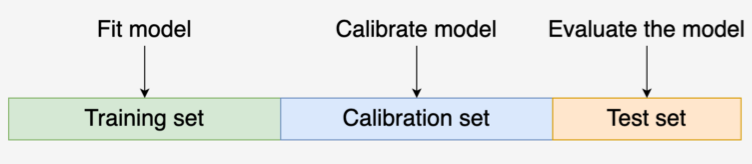
- Split data into Training, Calibration, and Test
- For each algorithm, train the algorithm on the Training set, and create the calibration model using it and the Calibration set.
- Each algorithm will have it’s own calibration model
- See below, Example: AdaBoost in Py using CV calibrator
- I like sklearn’s ideas for training a calibration model
- Use the Training set for CV or Nested CV
- For each split during CV or Nested CV (outer loop)
- Train the algorithm on the training fold, predict on the validation fold, calibrate predictions with calibration model, score the calibrated predictions for that fold
- The calibration model could be used in the tuning process in the inner loop of Nested CV as well
- Scores should include calibration metrics (See Diagnostics, Classification >> Calibration >> Basic Workflow)
- Train the algorithm on the training fold, predict on the validation fold, calibrate predictions with calibration model, score the calibrated predictions for that fold
- The rest is normal CV/Nested CV procedure
- i.e. average scores across the splits then select the algorithm with the best score. Predict and score algorithm on the Test set
- See Calibration curves for nested cv for details and code on averaging calibration curves
Methods
- Misc
- TLDR; Both Platt Scaling and Isotonic Regression methods are the essentially the same except:
- Platt Scaling uses a logistic regression model as the calibration model
- Isotonic Regression uses an isotonic regression model on ordered data as the calibration model
- TLDR; Both Platt Scaling and Isotonic Regression methods are the essentially the same except:
- Platt Scaling
Misc
- Suitable for smaller data and for calibration curves with the S-shape.
- May fail when model is already well calibrated (e.g. logistic regression models)
- Performs best under the assumption that the predicted probabilities are close to the midpoint and away from the extremes
- So, might be bad for tree models but okay for SVM, Naive Bayes, etc.
- This method, in its standard form, may not be appropriate after undersampling (Using Platt’s scaling for calibration after undersampling – limitations and how to address them)
- Performs a comparison between traditional Platt’s scaling, Platt’s scaling with the logit transformation, Platt’s scaling with a logistic GAM, Platt’s scaling with both the logit transformation and a logistic GAM, analytical calibration and isotonic regression.
- Conditions
- If Platt’s scaling would have been able to successfully calibrate the base model had it been trained on the entire dataset (i.e., without undersampling), then Platt’s scaling might be appropriate for calibration after undersampling.
- If this is not the case, a modified version of Platt’s scaling that fits a logistic GAM to the logit of the base model’s predictions is recommended.
Process
- Split data into Training, Calibration, and Test Sets
- Train your model on the Training Set
- Get the predicted probabilities from your model on the Test Set
- Fit a logistic regression using your model’s predicted probabilities for the Calibration Set as the predictor and the outcome variable in the Calibration Set as the outcome
- Calibrated probabilities are the predicted probabilities of the LR model using your model’s predicted probabilites on the Test set as new data.
Example: SVM in R
svm_platt_recal <- svm_platt_recal_func(model_fit, calib_dat, test_preds, test_dat) svm_platt_recal_func <- function(model_fit, calib_dat, test_preds, test_dat){ # Predict on Calibration Set cal_preds_obj <- predict(model_fit, calib_dat[, -which(names(calib_dat) == 'outcome_var')], probability = TRUE) # e1071 has a funky predict output; just getting probabilities cal_preds <- as.data.frame(attr(cal_preds_obj, 'probabilities')[, 2]) # Create calibration model cal_obs_preds_df <- data.frame(y = calib_dat$outcome_var, yhat = cal_preds[, 1]) calib_model <- glm(y ~ yhat, data = cal_obs_preds_df, family = binomial) # Recalibrate classifiers predicted probabilities on the test set colnames(test_preds) <- c("yhat") recal_preds = predict(calib.model, test_preds, type='response') return(recal_preds) }- See Istotonic Regression for “model_fit”, “calib_dat”, “test_preds”, and “test_dat”
Example: AdaBoost in py
X_, X_test, y_, y_test = train_test_split(X, y, test_size=0.3, random_state=42)
X_train, X_calib, y_train, y_calib = train_test_split(X_, y_, test_size=0.4, random_state=42)

# uncalibrated model
clf = AdaBoostClassifier(n_estimators=50)
y_proba = clf.fit(X_train, y_train).predict_proba(X_test)

# calibrated model
calibrator = LogisticRegression()
calibrator.fit(clf.predict_proba(X_calib), y_calib)
y_proba_calib = calibrator.predict_proba(y_proba)
- Isotonic Regression
More complex, requires a lot more data (otherwise it may overfit), but can support reliability diagrams with different shapes (is nonparametric).
- Tried on palmer penguins (n = 332) and almost all the probabilites were pushed to the edges
- Tried on mlbench::PimaIndiansDiabetes (n = 768). Probabilites were mostly clumped into 3 modes.
- Paper used a simulated (n = 5000) dataset. Probabilities moved a little more towards the center but the movement was much less dramatic that the other two datasets.
- I didn’t calculate brier scores but I’d guess you’d need over a 1000 or so observations for this method to have a significantly positive effect.
Lacks continuousness, because the fitted regression function is a piecewise function.
- So, a slight change in the uncalibrated predictions can result in dramatic difference in the calibrated predictions (i.e. a change in step)
Process
- Splits: train (50%), Calibration (25%), Test (25%)
- Train classifier model on train data
- Get predictions from the classifier on the test data
- Create calibration model dataset from the calibration data
- Get predictions from the classifier on the calibration data
- Create df with observed outcome of calibration data and predictions on calibration data
- Order df rows according the predictions column
- Lowest to largest probabilities in the paper but I’m not sure it matters
- FIt calibration model
- Fit isotonic regression model on calibration model dataset
- Create a step function using the isotonic regression fitted values and the predictions on the calibration data
- Calibrate the classifier’s predictions on the test set with the step function
Example: SVM in R
library(dplyr) library(e1071) data(PimaIndiansDiabetes, package = "mlbench") # isoreg doesn't handle NAs # e1071::svm doesn't identify the event correctly in non-0/1 factor variables dat_clean <- PimaIndiansDiabetes %>% mutate(diabetes = ifelse(as.numeric(diabetes) == 2, 1, 0)) %>% rename(outcome_var = diabetes) %>% tidyr::drop_na() # Data splits Training, Calibration, Test (50% - 25% - 25%) smp_size <- floor(0.50 * nrow(dat_clean)) val_smp_size = floor(0.25 * nrow(dat_clean)) train_idx <- sample(seq_len(nrow(dat_clean)), size = smp_size) train_dat <- dat_clean[train_idx, ] test_val_dat <- dat_clean[-train_idx, ] val_idx <- sample(seq_len(nrow(test_val_dat)), size = val_smp_size) calib_dat <- test_val_dat[val_idx, ] test_dat <- test_val_dat[-val_idx, ] rm(list=setdiff(ls(), c("train_dat", "calib_dat", "test_dat"))) # Fit classifier; predict on Test Set # e1071::svm needs a factor outcome, probability=T to output probabilities model_fit <- svm(factor(outcome_var) ~ ., data = train_dat, kernel = "linear", cost = 10, scale = FALSE, probability = TRUE) test_preds_obj <- predict(model_fit, test_dat[, -which(names(test_dat) == 'outcome_var')], probability = TRUE) # e1071 has a funky predict output; just getting probabilities test_preds <- as.data.frame(attr(test_preds_obj, 'probabilities')[, 2]) # Predict on Calibration Set cal_preds_obj <- predict(model_fit, calib_dat[, -which(names(calib_dat) == 'outcome_var')], probability = TRUE) # e1071 has a funky predict output; just getting probabilities cal_preds <- as.data.frame(attr(cal_preds_obj, 'probabilities')[, 2]) # Create Calibration Model dataset cal_obs_preds_mtx = cbind(y = calib_dat$outcome_var, yhat = cal_preds[, 1]) # order training data by predicted probabilities iso_train_mtx <- cal_obs_preds_mtx[order(cal_obs_preds_mtx[, 2]), ] # Fit Calibration Model # (predicted probabilities, observed outcome) calib_model <- isoreg(iso_train_mtx[, 2], iso_train_mtx[, 1]) # yf are the fitted values of the outcome variable stepf_data <- cbind(calib_model$x, calib_model$yf) step_func <- stepfun(stepf_data[, 1], c(0, stepf_data[, 2])) # recalibrate classifiers predicted probabilities on the test set recal_preds <- step_func(test_preds[, 1]) head(recal_preds, n = 20) hist(recal_preds) hist(test_preds[, 1])isoregdoesn’t handle NAs- For a binary classification model that outputs probabilities,
e1071::svmneeds:- factored 0/1 outcome variable
- probability = TRUE
Example: AdaBoost in Py using CV calibrator
from sklearn import datasets from sklearn import metrics from sklearn.model_selection import train_test_split from sklearn.ensemble import AdaBoostClassifier from sklearn.calibration import CalibratedClassifierCV from sklearn.model_selection import cross_val_predict from sklearn_evaluation import plot X, y = datasets.make_classification(10000, 10, n_informative=8, class_sep=0.5, random_state=42) X_train, X_test, y_train, y_test = train_test_split(X, y, test_size=0.3, random_state=42) clf = AdaBoostClassifier(n_estimators=100) clf_calib = CalibratedClassifierCV(base_estimator=clf, cv=3, ensemble=False, method='isotonic') clf_calib.fit(X_train, y_train) y_proba = clf_calib.predict_proba(X_test) y_proba_base = clf.fit(X_train, y_train).predict_proba(X_test) fig, ax = plt.subplots() plot.calibration_curve(y_test, [y_proba_base[:, 1], y_proba[:, 1]], clf_names=["Uncalibrated", "Calibrated"], n_bins=20) fig.set_figheight(4) fig.set_figwidth(6) fig.set_dpi(150)CalibratedClassifierCVhas both platt scaling (“sigmoid”)(default) and isotonic (“isotonic”) calibration methods (Docs)- Calibration model is built using the test fold (aka validation fold)
ensemble=True- For each cv split, the base estimator is fit on the training fold, and the calibration model is built using the “test” fold (aka validation fold)
- The test (aka validation) fold is the calibration data described in the isotonic and platt scaling process sections above
- For prediction, predicted probabilities are averaged across these individual calibrated classifiers.
- For each cv split, the base estimator is fit on the training fold, and the calibration model is built using the “test” fold (aka validation fold)
ensemble=False- LOO CV is performed using
cross_val_predict, and those predictions are used to train the calibration model. - The base estimator is trained using all the data (i.e. training and test (aka validation)).
- For prediction, there is only one classifier and calibration model combo.
- The benefit is that it’s faster, and since there’s only one combo, it’s smaller in size as compared to ensemble = True which is k combos. (not as accurate or as well-calibrated though)
- LOO CV is performed using
- Other forms
- For logistic regression models, adjustment using the Calibration Intercept (and Calibration Slope)
- Seems similar to Platt Scaling, but has strong overfitting vibes so caveat emptor
- For calculating the values, see Diagnostics, Classification >> Calibration >> Evaluation of Calibration Levels >> Weak >> Intercept, Slope
- See supplemental material in Calibration: the Achilles heel of predictive analytics
- Procedure
- The calibration intercept is added to the fitted model’s intercept
- The calibration slope is multiplied times all (nonexponentiated) coefficients of the fitted model (including interactions)
- Predictions are then calculated using the new formula
- Example
- From How We Built Our COVID-19 Estimator
- Target: Risk of Death (probabilities)
- Predictors: Age, Gender, Comorbidities
- Model: XGBoost
- “Every time our model makes a prediction, we compare the result to what the model would have returned for an individual of the same age and sex and only one of the listed comorbidities, or none at all. If the predicted risk is lower than the risk for a comorbidity taken on its own—such as, say, the estimated risk for heart disease alone being greater than the risk for heart disease and hypertension, or the risk for metabolic disorders being lower than the risk of someone with no listed comorbidities—our tool delivers the higher number instead. We also smoothed our estimates and confidence intervals, using five-year moving averages by age and gender.”
- For logistic regression models, adjustment using the Calibration Intercept (and Calibration Slope)
Feature Importance
Misc
- Also see
- My notebook and bookmarks for proper algorithms (e.g. permutation importance) to specify for variable importance plots
- Diagnostics, Model Agnostic for various feature importance computations
- Packages
- {diversityForest} (Paper) - Calculates multi-class VIM which is tailored for identifying exclusively class-associated covariates. It measures the discriminatory ability of the splits performed in the respective covariates with regard to this split criterion
- Fits multi forests (MuFs) that use both multi-way and binary splitting. The multi-way splits generate child nodes for each class, using a split criterion that evaluates how well these nodes represent their respective classes.
- MuFs are primarily useful for the VIM calculations as they often have slightly lower predictive performance compared to conventional RFs
- Also includes a discriminatory VIM, based on the binary splits, that assesses the strength of the general influence of the covariates, irrespective of their class-associatedness.
- Fits multi forests (MuFs) that use both multi-way and binary splitting. The multi-way splits generate child nodes for each class, using a split criterion that evaluates how well these nodes represent their respective classes.
- {lvimp} - Variable importance of variables for predicting the response at each time point and the importance summarized over the time series. (longitudinal setting)
- {rfPermute} - Estimate Permutation p-Values for Random Forest Importance Metrics
- {vip} - Part of IML suite of packages. See Diagnostics, Model Agnostic, >> IML
- {vimp} - Computes algorithm-agnostic estimates of population variable importance, along with asymptotically valid confidence intervals for the true importance and hypothesis tests of the null hypothesis of zero importance
- Types:
- Difference in population Classification Accuracy
- Difference in population AUROC
- Difference in population Deviance,
- Difference in population R2
- None of the vignettes describe the algorithm. The authors provide links to papers for more details, but the freely available ones look pretty dense.
- I recommend checking out this paper, A Guide to Feature Importance Methods for Scientific Inference >> Section 10, Statistical Inference for FI Methods >> WVIM including LOCO for a brief description of the {vimp}’s method. Also see other parts of the paper have details on WVIM and LOCO.
- Types:
- {xplainfi} - Feature Importance Methods for Global Explanations
- Includes permutation feature importance (PFI), conditional and relative feature importance (CFI, RFI), leave one covariate out (LOCO), and Shapley additive global importance (SAGE), as well as feature sampling mechanisms to support conditional importance methods
- {diversityForest} (Paper) - Calculates multi-class VIM which is tailored for identifying exclusively class-associated covariates. It measures the discriminatory ability of the splits performed in the respective covariates with regard to this split criterion
- Compute Feature Importance (FI) values on test data only. Computing on training data may lead to wrong conclusions. (source)
- Permutation Importance
- Permutation importance is generally considered as a relatively efficient technique that works well in practice
- Importance of correlated features may be overestimated
- If you have highly correlated features, use
partykit::varimp(conditional = TRUE)
- If you have highly correlated features, use
- Process
- Take a model that was fit to the training dataset
- Estimate the predictive performance of the model on an independent dataset (e.g., validation dataset) and record it as the baseline performance
- For each feature i:
- randomly permute feature column i in the original dataset
- record the predictive performance of the model on the dataset with the permuted column
- compute the feature importance as the difference between the baseline performance (step 2) and the performance on the permuted dataset
- Variable Importance plots can be useful for explaining the model to clients. They should never be interpreted as causal. Ex. Real estate: variables that are most influential in determining housing price by this model are aspects of a house that could be emphasized by Realtors to their clients.
- Make sure to use “LossFunctionChange” importance type in Catboost.
- Looks at how much the loss function changes when a feature is excluded from the model.
- Default method capable of giving importance to random noise
- Requires evaluation on a testing set
- Also see
xgboost
xg_wf_best <- xg_workflow_obj %>%
finalize_workflow(select_best(xg_tune_obj))
xg_fit_best <- xg_wf_best %>%
fit(train)
importances <- xgboost::xgb.importance(model = extract_fit_engine(xg_fit_best))
importances %>%
mutate(Feature = fct_reorder(Feature, Gain)) %>%
ggplot(aes(Gain, Feature)) +
geom_point() +
labs(title = "Importance of each term in xgboost",
  subtitle = "Even after turning direction numeric, still not *that* important")
Using vip package
library(vip)

# xg_wf = xgboost workflow object
fit(xg_wf, whole_training_set) %>%
pull_workflow_fit() %>%
vip(num_features = 20)
glmnet
.png)
lin_trained <- lin_wf %>%
    finalize_workflow(select_best(lin_tune)) %>%
    fit(train) # or split_obj, test_dat, etc.

lin_trained$fit$fit %>%
    broom::tidy %>%
    top_n(50, abs(estimate)) %>%
    filter(term != "(Intercept)") %>%
    mutate(ter = fct_reorder(term, estimate)) %>%
    ggplot(aes(estimate, term, fill = estimate > 0)) +
    geom_col() +
    theme(legend.position = "none")