A suitably flexible Bayesian regression adjustment model,
Chosen by cross-validation/LOO,
Including Gaussian processes for the unit-level effects over time (and space/network if relevant),
Imputation of missing data, and
Informative priors for biases in the data collection process.
Discrete Parameters
Models with discrete parameters arise in a range of statistical motifs including hidden Markov models, finite mixture models, and generally in the presence of unobserved categorical data
HMC cannot operate on models containing discrete parameters. HMC relies on gradient information to guide its exploration of the parameter space. Discrete parameters don’t have well-defined gradients.
Using HMC would require marginalization of the likelihood to remove these discrete dimensions from the sampling problem (i.e. integrating out discrete variables).
This can result in loss of information
Depending on the number of discrete parameters, it can be computationally instensive or intractable.
The direct relationship between discrete parameters and the data is obscured.
Potentially requiring more samples to achieve the same level of accuracy due to slower mixing
Can be complex and error-prone for intricate models
{nimbleHMC} (JOSS) can perform HMC sampling of hierarchical models that also contain discrete parameters. It allows for HMC sampling operating alongside discrete samplers.
A workflow for a problem with discrete parameters should consist of testing combinations of samplers in order to optimize MCMC efficiency
{nimbleHMC} allows you to mix-and-match samplers from a large pool of candidates.
{compareMCMCs} (JOSS) - Compares MCMC Efficiency from ‘nimble’ and/or Other MCMC Engines
Built-in metrics include two methods of estimating effective sample size (ESS), posterior summaries such as mean and common quantiles, efficiency defined as ESS per computation time, rate defined as computation time per ESS, and minimum efficiency per MCMC.
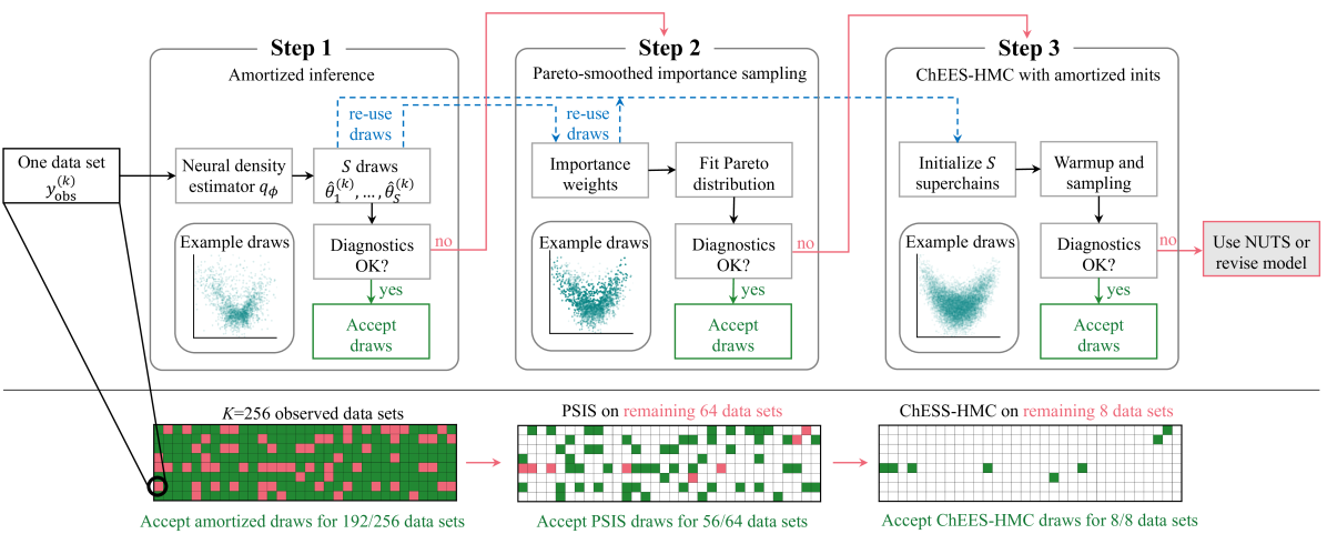
Amortized Bayesian Inference uses deep neural networks to learn a direct mapping from observables, \(y\), to the corresponding posterior, \(p(\theta | y)\)
i.e. Approximates posterior distributions for faster parameter estimation.
Popular for simulation-based inference (SBI) but is expanding beyond SBI
{{BayesFlow}} - A library for amortized Bayesian inference with neural networks.
Multi-backend via Keras 3: Use PyTorch, TensorFlow, or JAX.
Modern nets: Flow matching, diffusion, consistency models, normalizing flows, transformers
Built-in diagnostics and plotting
2-Stage Approach
Training Stage: neural networks learn to distill information from the probabilistic model based on simulated examples of observations and parameters, \((\theta | y) \sim p(\theta) \;p(y|\theta)\)
Inference Stage: neural networks approximate the posterior distribution for an unseen data set, \(y_\text{obs}\) in near-instant time without repeating the training stage
The sequential nature of MCMC creates a computational bottleneck as each step in the chain depends on the previous state, making parallelization difficult.
MCMC methods typically require evaluating the likelihood function using the entire dataset at each iteration.
Instead of sampling from the unknown posterior distribution, it is assumed that there exists a family of distributions \(Q\) that can approximate the unknown posterior, \(p(z|x)\)
The standard proposed distribution uses a mean-field approximation, in that it assumes that all latent variables are mutually independent. This assumption implies that the joint distribution factorizes into a product of marginal distributions, making computation more tractable.
The mean-field assumption implies that the posterior uncertainty of SVI tends to be underestimated (CIs too narrow)
Unlike MCMC which uses sampling, SVI formulates Bayesian inference as an optimization problem by minimizing the Kullback-Leibler (KL) divergence between our approximation and the true posterior
Research along this route tends to focus on two main directions: improving the variational family \(Q\) or developing better versions of the ELBO.
More expressive families like normalizing flows can capture complex posterior geometries but come with higher computational costs (Currently not suitable for larger datasets)
Normalizing Flows - A density estimation technique that chains together multiple diffeomorphisms \(\phi_1, \phi_2, \ldots, \phi_k\) to gradually obtain \(x\)(original data) coming from a complex distribution \(p_X(x)\), starting from \(u\), coming from a simple base distribution \(p_U(u)\) (e.g Gaussian).
Evidence Lower Bound (ELBO) - Maximizing this quantity is equivalent to minimizing the K-L divergence. (Done using stochasitic optimization)
Helps it to scale, but can come at the cost of some approximation quality