Geospatial
Misc
- Also see Geospatial, Spatial Weights
- Packages
- {waywiser} - Measures the performance of models fit to 2D spatial data by implementing a number of well-established assessment methods in a consistent, ergonomic toolbox
- Features include new yardstick metrics for measuring agreement and spatial autocorrelation, functions to assess model predictions across multiple scales, and methods to calculate the area of applicability of a model.
- {geospt} - Estimation of the variogram through trimmed mean, radial basis functions (optimization, prediction and cross-validation), summary statistics from cross-validation, pocket plot, and design of optimal sampling networks through sequential and simultaneous points methods.
- {geosptdb} - Spatio-Temporal Radial Basis Functions with Distance-Based Methods (Optimization, Prediction and Cross Validation)
- {spdep} - Spatial autocorrelation functions
- {sperrorest} - Implements spatial error estimation and permutation-based spatial variable importance using different spatial cross-validation and spatial block bootstrap methods, used by {mlr3spatiotempcv}.
- {waywiser} - Measures the performance of models fit to 2D spatial data by implementing a number of well-established assessment methods in a consistent, ergonomic toolbox
- Papers
Spatial Autocorrelation
- Misc
- Also see Association, Spatial
- Residual spatial autocorrelation has an effect of standard errors and on coefficient values.
- Testing the residuals of intercept-only or other simple (few or irrelevant covariates) models will erroneously detect patterns as (global) spatial autocorrelation.
- i.e. a significant Moran’s I doesn’t necessarily mean you need spatial econometrics (lags, modelled errors) — it might just mean your model is missing a spatially-patterned covariate.
- See Misc >> Causes of Spurious Spatial Autocorrelation >> Omitted Variables for more details
- Visual Assessment
Also see Association, Spatial >> Local Measures >> Examples >> Example 3 >> lm.multivariable
Example: (source)
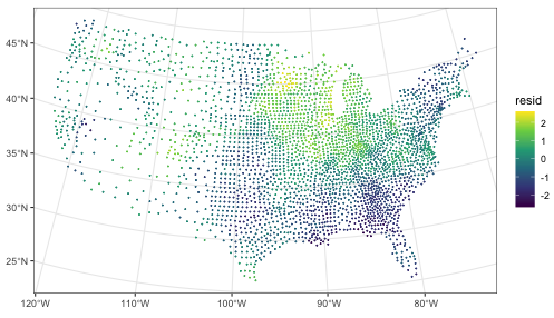
libary(ggplot2) data("US_counties_centroids", package = "SpatialInference") spuriouslm <- fixest::feols( noise1 ~ noise2, data = US_counties_centroids, vcov = "HC1" # robust SEs ) spuriouslm #> OLS estimation, Dep. Var.: noise1 #> Observations: 3,108 #> Standard-errors: Heteroskedasticity-robust #> Estimate Std. Error t value Pr(>|t|) #> (Intercept) 6.890000e-16 0.017872 3.860000e-14 1.0000e+00 #> noise2 8.738022e-02 0.015535 5.624836e+00 2.0216e-08 *** #> --- #> Signif. codes: 0 '***' 0.001 '**' 0.01 '*' 0.05 '.' 0.1 ' ' 1 #> RMSE: 0.996015 Adj. R2: 0.007316 US_counties_centroids$resid <- spuriouslm$residuals ggplot(US_counties_centroids) + geom_sf(aes(col = resid), size = .1) + theme_bw() + scale_color_viridis_c()- noise1 and noise2 are independent of each other but spatially coorelated. This leads to an inflated t-value and low p-value.
- Clustering of high residuals in the Midwest
- Moran’s I
- See Association, Spatial >> Global >> Moran’s I
- The saddlepoint approximation is the best version
- {spdep::lm.morantest}
resfun takes residuals, weighted.residuals (default), rstandard, or rstudent
Example:
library(spdep) data(pol_pres15, package = "spDataLarge") pol_pres15 <- pol_pres15 |> janitor::clean_names() # neighbor list and spatial weights nb_poly_pol <- pol_pres15 |> poly2nb(queen = TRUE) lw_b_poly_pol <- nb_poly_pol |> nb2listw(style = "B") moran_lookup <- c( morans_i = "estimate1", expectation = "estimate2", variance = "estimate3", std.deviate = "statistic" ) lm(i_turnout ~ 1, pol_pres15) |> lm.morantest(listw = lw_b_poly_pol) |> broom::tidy() |> rename(any_of(moran_lookup)) |> relocate(method, alternative, everything()) #> # A tibble: 1 × 7 #> method alternative morans_i expectation variance std.deviate p.value #> <chr> <chr> <dbl> <dbl> <dbl> <dbl> <dbl> #> 1 Global Moran I for regression residuals greater 0.691 -0.000401 0.000140 58.5 0- The intercept-only model is equivalant to
moran.test(response_var, randomisation = FALSE) - p-value < 0.05, so spatial autocorrelation is present
- The intercept-only model is equivalant to
- Other flavors
- Rao’s Score
- Estimates of tests chosen among five statistics for testing for spatial dependence
- See Regression, Spatial >> Econometric >> Diagnostics >> Rao’s Score
- {spdep::lm.RStests}