Preprocessing
Misc
- Packages
- {apache.sedona} - Sparklyr extension for processing geospatial data
Example: Larger-than-memory spatial/KNN join
Code
import sedona.db sd = sedona.db.connect() sd.options.memory_limit = "3g" sd.options.memory_pool_type = "fair" url = "https://github.com/geoarrow/geoarrow-data/releases/download/v0.2.0/microsof" sd.read_parquet(url).to_view("buildings") sd.sql(""" SELECT ROW_NUMBER() OVER () AS building_id, geometry FROM buildings """).to_parquet("buildings_idx.parquet") sd.sql(""" SELECT l.building_id, r.building_id AS nearest_building_id, l.geometry AS geometry, ST_Distance(l.geometry, r.geometry) AS dist FROM "buildings_idx.parquet" AS l JOIN "buildings_idx.parquet" AS r ON l.building_id <> r.building_id """)- Requires setting a memory limit
- {chopin} - Automates parallelization in spatial operations with chopin functions as well as sf/terra functions.
- Raster resolution: Suggests 100 meters as a threshold. Rasters with resolution coarser than 100 meters and a few layers would be better for the direct call of
exactextractr::exact_extract. - Set
sf::sf_use_s2(FALSE)- Works best with two-dimensional (planar) geometries. Running any chopin functions at spherical or three-dimensional (e.g., including M/Z dimensions) geometries may produce incorrect or unexpected results.
- Raster resolution: Suggests 100 meters as a threshold. Rasters with resolution coarser than 100 meters and a few layers would be better for the direct call of
- {geographiclib} - R interface to GeographicLib for precise geodetic calculations on the WGS84 ellipsoid
- Geodesic computations (distance, bearing, paths, intersections)
- Map projections (UTM/UPS, Transverse Mercator, Lambert Conformal Conic, and more)
- Grid reference systems (MGRS, Geohash, GARS, Georef)
- Coordinate conversions (geocentric, local Cartesian)
- Polygon area on the WGS84 ellipsoid
- {photon} - High-Performance Geocoding using photon
- {apache.sedona} - Sparklyr extension for processing geospatial data
- Resources
- Geocomputation with R, Ch.8 File Formats
- Conflation Types (i.e. geospatial joins)
- Notes fromConflating Overture Places Using DuckDB, Ollama, Embeddings, and More
- Recommends using String Similarity. Then use Embeddings on the remaining unmatched. Shows an 80% match. Can get about 90% by raising the similarity threshold, but it increases the amount of false positive matches.
- Exact Name Matching (e.g. by name variable
- Article example had a ~31% match rate
- String Similarity (e.g. address variable + Jaro-Winkler distance)
- Article example had a ~68% match rate
- Embeddings (e.g. embed name variable + cosine similarity)
- Article example had a ~71% match rated
- Notes fromConflating Overture Places Using DuckDB, Ollama, Embeddings, and More
File Types
GeoPackage - Defined as a SQLite 3 database file with a specific database schema and with filename extension
.gpkg. The schema defines data and metadata tables with specified definitions, integrity assertions, format limitations and content constraints (wiki)Designed to be as lightweight as possible and be contained in one ready-to-use single file. This makes it suitable for mobile applications in disconnected mode and rapid sharing on cloud storage, USB drives, etc.
The GeoPackage extension F.3 RTree Spatial Indexes specifies how to use SQLite spatial indexes in order to speed up performance on spatial queries compared to traditional geospatial files formats.
Example: Writing (source)
phoenician |>
  st_write(
    "data/phoenician_settlements.gpkg",
    layer = "phoenician_settlements",
    layer_options = c(
      "IDENTIFIER=Phoenician colonization from its origin to the 7th century BC",
      glue("DESCRIPTION=Data from:
            Manzano-Agugliaro, F., Marín-Buzón, C., Carpintero-Lozano, S., & López-Castro, J. L. (2025). \\
            Phoenician colonization from its origin to the 7th century BC. Journal of Maps, 21(1). \\
            https://doi.org/10.1080/17445647.2025.2528876

            Available on https://doi.org/10.5281/zenodo.17141060

            Extracted on {Sys.Date()} – https://r.iresmi.net/posts/2025/phoenician")),
    delete_layer = TRUE,
    quiet = TRUE)
PMTiles - A single-file archive format for tiled data. A PMTiles archive can be hosted on a commodity storage platform such as S3, and enables low-cost, zero-maintenance map applications that are “serverless” - free of a custom tile backend or third party provider. (Docs)
- Packages
- {freestiler} - A tiling engine that is written in Rust and optimized for speed and performance.
- Generate tiles directly from R sf objects and Python GeoDataFrames.
- DuckDB integration supports local DuckDB databases, GeoParquet files, and even shapefiles
- Default output is MapLibre Tiles (MLT) (packaged as PMTiles) which is a next-generation tile format that optimizes for performance and data compression
- {pmtiles}
- {freestiler} - A tiling engine that is written in Rust and optimized for speed and performance.
- Run your interactive, smooth-zooming vector map from any storage like S3 that supports http requests; a Caddy server running on your Wi-Fi router, or even GitHub pages (if tiles < 1GB).
- Cloudflare R2 is the recommended storage platform for PMTiles because it does not have bandwidth fees, only per-request fees: see R2 Pricing.
- Resources
- Example loading pmtiles and using w/{mapgl}
- Complete project using vehicle trends data.
- Creates PMTiles using {pmtiles} from parquet data
- Directions for uploading pmtiles to cloudflare r2
- Hosts on github pages
- Packages
Reading/Writing
Geopackage
Check for available layers, Read, and Write
st_layers("path/to/nc.gpkg") # Driver: GPKG # Available layers: # layer_name geometry_type features fields crs_name # 1 nc.gpkg Multi Polygon 100 14 NAD27 nc <- st_read("path/to/nc.gpkg") # Reading layer `nc.gpkg' from data source # `/home/edzer/R/x86_64-pc-linux-gnu-library/4.4/sf/gpkg/nc.gpkg' # using driver `GPKG' # Simple feature collection with 100 features and 14 fields # Geometry type: MULTIPOLYGON # Dimension: XY # Bounding box: xmin: -84.3 ymin: 33.9 xmax: -75.5 ymax: 36.6 # Geodetic CRS: NAD27 st_write( nc, "path/to/nc.gpkg", layer = "layer_nc" )- append: Allows
st_writeto either append records to an existing layer or replace it
- append: Allows
GeoJSON
Write data to geojson
data %>%
    st_write("mb_shapes.geojson")
CSV to Dataframe (source)
# points localidad <- st_as_sf(localidad, coords = c("longitude", "latitude"), crs = 4326) # polygons departamentos <- st_as_sf(departamentos, wkt = "geomTDepartamento")- wkt is the column that holds WKT encoded geometries
Dataframe to CSV (source)
phoenician |>
  select(-c(latitude_n, longitude_e)) |>
  bind_cols(st_coordinates(phoenician)) |>
  rename(lon_wgs84 = X,
         lat_wgs84 = Y) |>
  st_drop_geometry() |>
  write_csv("data/phoenician_settlements.csv")
Shape Files
Read in only the attributes table using
foreign::read.dbfif you don’t need the geometries (source)Read in the full spatial data and drop the geometry using
sf::st_drop_geometryorterra::values(source)- These pull out the data frame, so if you assigned it to a different object you have to remove the spatial object
Validate geometries when loading a shape file
NY8_sf <- st_read(system.file( "shapes/NY8_bna_utm18.gpkg", package = "spData"), quiet = TRUE) # validate geometries table(st_is_valid(NY8_sf)) #> TRUE #> 281- If
st_is_validreturns FALSE, then you can runst_make_valid
- If
Example: Counties in California
tbl <- tigris::counties(state = "CA") %>% st_set_crs(4326){tigris} - US data
library(tigris) us_states <- states(resolution = "20m", year = 2022, cb = TRUE) lower_48 <- us_states %>% filter(!(NAME %in% c("Alaska", "Hawaii", "Puerto Rico"))){rnaturalearth} - World data
# Via URL
# Medium scale data, 1:50m Admin 0 - Countries
# Download from https://www.naturalearthdata.com/downloads/50m-cultural-vectors/
world_map <- read_sf("ne_50m_admin_0_countries/ne_50m_admin_0_countries.shp") %>%
  filter(iso_a3 != "ATA")  # Remove Antarctica

# Via Package
library(rnaturalearth)

# rerturnclass = "sf" makes it so the resulting dataframe has the special
# sf-enabled geometry column
world_map <- ne_countries(scale = 50, returnclass = "sf") %>%
  filter(iso_a3 != "ATA")  # Remove Antarctica
Big Data
Misc
- If your computation takes in the 30 sec to a few minutes range, then use duckdb and its spatial extensions (See Databases, DuckDB >> Geospatial, Apache >> Arrow >> Misc >> {geoarrow})
- If your compution take closer to 10 to 20 minutes or more, then use Apache Sedona (See package in Misc)
- Sedona can do parallelized joins.
- geoparquet (vector) and COGS (raster) allow users to only download what they need and not the entire set of files.
Fast read
library(vapour)
library(geos)
elevation <- vapour_read_geometry("data/ns-water_elevation.fgb") |>
  geos_read_wkb(crs = st_crs(lakes))
Use a SQL query to reduce the data read into memory (source)
With {sf} and with a bounding box
high_capacity <- read_sf( url, wkt_filter = wkt_bdd, query = "SELECT * FROM wind_turbine WHERE Turbine_Rated_Capacity__kW_ > 4000" )- wind_turbine is a layer discovered using
st_layersin the previous example
- wind_turbine is a layer discovered using
With {terra}
f <- system.file("ex/lux.shp", package="terra")
v <- vect(f)
v
#>  class       : SpatVector
#>  geometry    : polygons
#>  dimensions  : 12, 6  (geometries, attributes)
#>  extent      : 5.74414, 6.528252, 49.44781, 50.18162  (xmin, xmax, ymin, ymax)
#>  source      : lux.shp
#>  coord. ref. : lon/lat WGS 84 (EPSG:4326)
#>  names       :  ID_1   NAME_1  ID_2   NAME_2  AREA       POP
#>  type        : <num>    <chr> <num>    <chr> <num>     <num>
#>  values      :     1 Diekirch     1 Clervaux   312 1.808e+04
#>                    1 Diekirch     2 Diekirch   218 3.254e+04
#>                    1 Diekirch     3  Redange   259 1.866e+04
v <-
  vect(f,
       query="SELECT NAME_1, NAME_2, ID_2 FROM lux WHERE ID_2 < 4")
Use lazy evaluation via {terra}
As a SpatVectorProxy
f <- system.file("ex/lux.shp", package="terra") v <- vect(f, proxy=TRUE) v #> class : SpatVectorProxy #> geometry : polygons #> dimensions : 12, 6 (geometries, attributes) #> extent : 5.74414, 6.528252, 49.44781, 50.18162 (xmin, xmax, ymin, ymax) #> source : lux.shp #> coord. ref. : lon/lat WGS 84 (EPSG:4326) #> names : ID_1 NAME_1 ID_2 NAME_2 AREA POP #> type : <num> <chr> <num> <chr> <num> <num> summary(v) # reads only metadata v[1:5, ] # reads just a few features x <- query(v, vars=c("ID_2", "NAME_2"), start=5, n=2) x #> class : SpatVector #> geometry : polygons #> dimensions : 2, 2 (geometries, attributes) #> extent : 5.74414, 6.528252, 49.72324, 50.03632 (xmin, xmax, ymin, ymax) #> source : lux.shp #> coord. ref. : lon/lat WGS 84 (EPSG:4326) #> names : ID_2 NAME_2 #> type : <num> <chr> #> values : 5 Wiltz #> 6 Echternach- Using proxy = TRUE, allows you to reference a spatial vector dataset (like a shapefile or GeoPackage layer) without actually reading all the data into memory. This is especially useful when working with large datasets that don’t fit comfortably into RAM.
Reduce Size Via SQL Query
Uses OGR SQL (SQLite might also be accepted)
Choose Layer
library("sf") st_layers("data/Lower_layer_Super_Output_Areas_2021_EW_BGC_V3.gpkg") ## Driver: GPKG ## Available layers: ## layer_name geometry_type features fields crs_name ## 1 LSOA_2021_EW_BGC_V3 Multi Polygon 35672 7 OSGB36 / British National Grid- This file only has one layer
Get an idea of the columns in the layer by looking at the first row.
st_read("data/Lower_layer_Super_Output_Areas_2021_EW_BGC_V3.gpkg", query = "SELECT * FROM LSOA_2021_EW_BGC_V3 WHERE FID = 1", quiet = TRUE) ## Simple feature collection with 1 feature and 7 fields ## Geometry type: MULTIPOLYGON ## Dimension: XY ## Bounding box: xmin: 531948.3 ymin: 181263.5 xmax: 532308.9 ymax: 182011.9 ## Projected CRS: OSGB36 / British National Grid ## LSOA21CD LSOA21NM BNG_E BNG_N LONG LAT ## 1 E01000001 City of London 001A 532123 181632 -0.09714 51.51816 ## GlobalID SHAPE ## 1 {1A259A13-A525-4858-9CB0-E4952BA01AF6} MULTIPOLYGON (((532105.3 18...- FID = 1 says look at the first row. FID is the feature ID attribute. I don’t think it’s actual column in the dataset.
Query the layer and filter
st_read("data/Lower_layer_Super_Output_Areas_2021_EW_BGC_V3.gpkg", query = "SELECT * FROM LSOA_2021_EW_BGC_V3 WHERE LSOA21CD LIKE 'W%'", quiet = TRUE)- W% says looks for values that start with “W” (Wales) in the LSOA21CD column
- Based on the OCR SQL docs I think
%is wildcard for multiple characters.
- Based on the OCR SQL docs I think
- W% says looks for values that start with “W” (Wales) in the LSOA21CD column
Use a bounding box to filter overlapping geometries
Example: Filter polygons overlapping the boundaries of Wales
Filter Wales from a UK shapefile dataset
uk <- sf::st_read("data/Countries_December_2022_GB_BGC.gpkg")
wales <- dplyr::filter(uk, CTRY22NM == "Wales")
Create Wales polygon
wales_wkt <-
  wales |>
  sf::st_geometry() |>
  sf::st_as_text()
Filter overlapping geometries
wales_lsoa <- sf::st_read("data/Lower_layer_Super_Output_Areas_2021_EW_BGC_V3.gpkg", wkt_filter = wales_wkt)- Some English LSOAs along the Wales/England border in addition to the Welsh LSOAs are read in, because these technically overlap with the Wales polygon on the border itself. Not perfect but still reduces the data being read into memory.
Projections
Misc
- Packages
- {crstools} - Choose the appropriate map projection for a given application, visualise the resulting distortion, and georeference data from unknown projections
- {parzer} - Parses messy geographic coordinates
Example:
data("wind", package = "gstat")
as.character(wind.loc[["Latitude"]][[1]])
#> [1] "51d56'N"

as.numeric(sp::char2dms(as.character(
  wind.loc[["Latitude"]][[1]]
)))
#> [1] 51.93333

parzer::parse_lat(as.character(
  wind.loc[["Latitude"]][[1]]
))
#> [1] 51.93333
- Resources
- Google “epsg code” + “your region name” to find a reasonable projection code to use
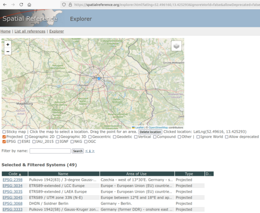
- Spatial Reference
- Valid longitude should be between -180 and 180 (or 0-360 for some systems)
- Valid latitude should be between -90 and 90.
- Formats
- epsg: The EPSG code (if available), a standardized code for coordinate systems.
- proj4string: A text string defining the projection parameters in PROJ.4 format.
- wkt: The Well-Known Text representation of the CRS.
- OGC (Open Geospatial Consortium) vs WGS (World Geodetic System)
- Both are same except for axis order
- WGS84 (EPSG:4326) uses latitude/longitude order (y,x)
- Traditional axis order used by cartographers and geographers throughout history
- CRS84 (OGC:CRS84) uses longitude/latitude order (x,y)
- Adopted since many mathematical and computational systems conventionally list x first, then y.
- Example:
st_transform(data, "OGC:CRS84")
- With data that’s in an older coordinate system, transformation instructions to a more modern system might be included in the output (wkt text) of the
st_crs- SOURCECRS: Your actual current coordinate system (e.g. UTM Zone 18N with Clarke 1866 datum)
- TARGETCRS: The reference system you’ll be in after the transformation (e.g. WGS84)
- ABRIDGEDTRANSFORMATION: Instructions for converting between the source and target systems
Geographic Coordinates
AKA geodetic coordinates, ellipsoidal
X → Longitude (east–west)
Y → Latitude (north–south)
Required for Great Distance and Spherical Distance calculations
EPSG:4326 (WGS 84)
Usage Area: World
Most common for global datasets. Used by most web mapping services and GPS devices
Required by leaflet
Formats
st_transform(data, "EPSG:4326")    # Most common
st_transform(data, "WGS84")        # Also works
st_transform(data, "+proj=longlat +datum=WGS84")  # Seen in older code before epsg
st_transform(data, 4326)           # epsg value
EPSG:4269 (NAD83):
Official US standard: NAD83 is the official horizontal datum used by US federal agencies and most state/local governments for mapping and surveying within the continental United States.
Specifically designed for North America and provides slightly better positional accuracy for the continental US than WGS84.
Convert dataframe with latitude and longitude to a sf object with geometries
new_tbl <- old_tbl # contains latitude and longitude variables
    # convert to simple features object
    sf::st_as_sf(
        coords = c("<longitude_var>", "<latitude_var>"), # order matters
        crs = 4326
    ) %>%
    mapviw::mapview()
Transform a sf object to WSG84 coordinates
us_states <- us_states %>% # df with geometries
  sf::st_transform("EPSG:4326")  # WGS 84
Projected Coordinates
aka cartesian
Used for Planar Distance calculations
X → Easting (distance east from the zone’s central meridian, usually in meters)
Y → Northing (distance north from the equator, usually in meters)
Packages
- {albersusa} - Tools, Shapefiles & Data to Work with an ‘AlbersUSA’ Composite Projection
United States:
- States
- Each state also has its own State Plane coordinate system
- States also have zones that zoom into a particular region of the state. Each will have it’s own EPSG.
- Alaska has 10 zones (most of any state)
- Texas has 5 zones
- California has 6 zones
- Florida has 3 zones
- Rhode Island has just 1 zone (like many smaller states)
- There also are separate projections for feet and meters
- Example: Hawaii Zone 3
- EPSG:6633, NAD83(PA11) / Hawaii zone 3 (feet)
- EPSG:6630, NAD83(PA11) / Hawaii zone 3 (meters)
- Example: Hawaii Zone 3
- Hawaii EPSG:6320 NAD83(PA11)
- Alaska EPSG:6393: NAD83(2011)
- Continental/Contiguous US (CONUS), i.e. 48 states:
- Use EPSG:6350 as it is the most current and most accurate
- Timeline on the CONUS projections
- EPSG:5069: NAD27 / Conus Albers; Replaced by NAD83 EPSG:5070
- EPSG:5070: NAD83 / Conus Albers; For applications with an accuracy of better than 1m, replaced by NAD83(HARN) EPSG:5071
- EPSG:5071: NAD83(HARN) / Conus Albers; Replaced by NAD83(NSRS2007) EPSG:5072
- EPSG:5072: NAD83(NSRS2007) / Conus Albers
- EPSG:6350: NAD83(2011) / Conus Albers; Replaces NAD83(NSRS2007) / Conus Albers
- Snyder’s GS48 (StackEx, Example): Not sure how its accuracy compares to NAD83, but it looks good on a map.
- Only supported via proj string,
st_transform(crs = "+proj=gs48")
- Only supported via proj string,
- North American Terrestrial Reference Frame of 2022 (NATRF2022). These new datums will replace NAD83 and are expected to be released in 2025. Once these datums are adopted, new projections (e.g., Albers or UTM) will likely be defined for CONUS using the updated reference frames.
- States
Europe:
- Pan-Europe, European Union
- EPSG:3035 - ETRS89-LAEA
- Central Europe (between 6°E and 12°E) (Think Western Nordic, Denmark, Germany, Northern Italy)
- EPSG:25832 - Uses datum ETRS89 and UTM zone 32N projection
- Preferred standard for European mapping applications.
- EPSG:32632 - Uses datum WGS84 and UTM zone 32N projection
- EPSG:25832 - Uses datum ETRS89 and UTM zone 32N projection
- Individual countries often have their own systems
- e.g. British National Grid OSGB36 (EPSG:27700)
- Pan-Europe, European Union
NAD83, Albers, Mercator, Robinson
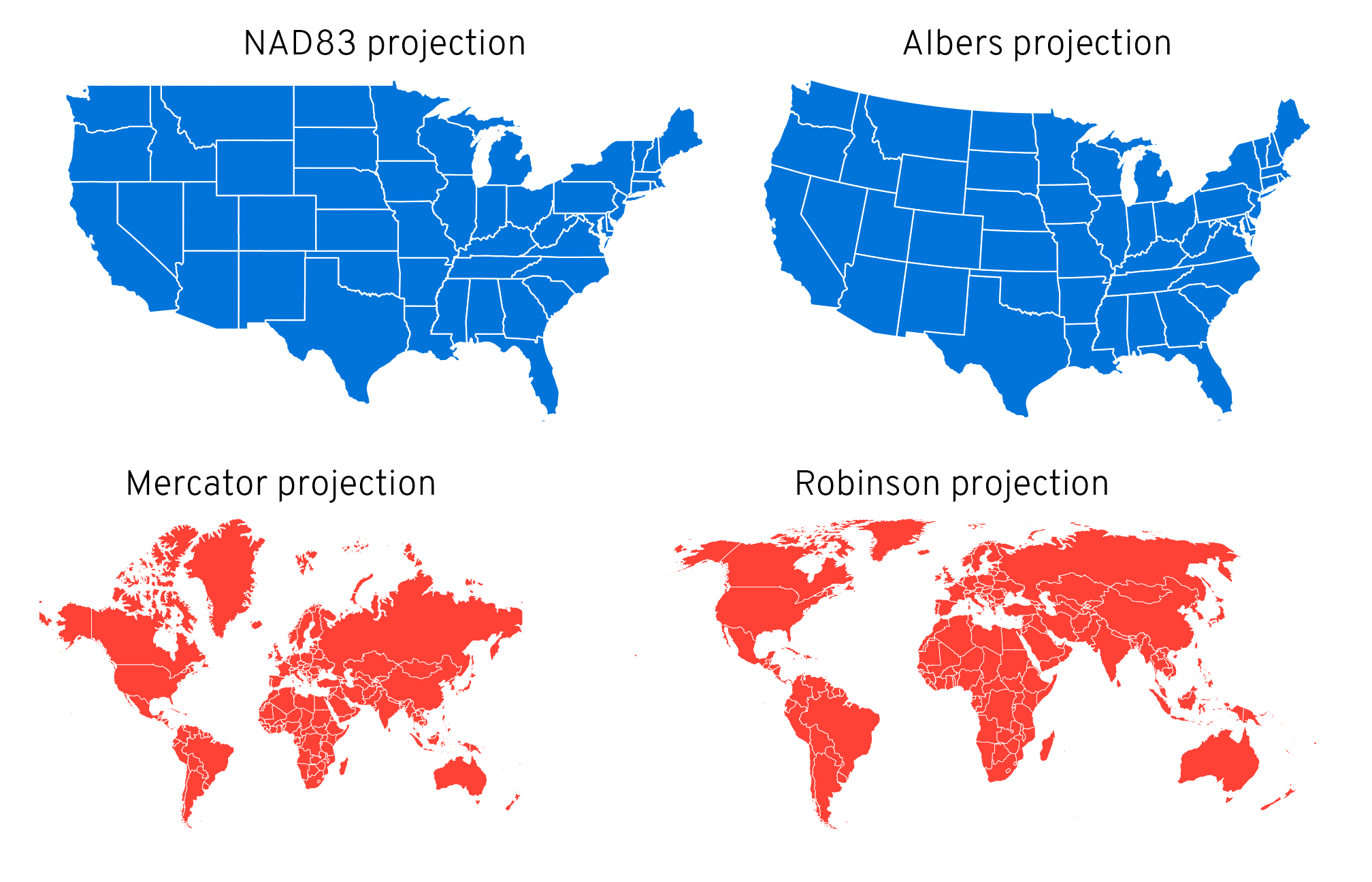
library(patchwork)

p1 <- ggplot() +
  geom_sf(data = lower_48, fill = "#0074D9", color = "white", linewidth = 0.25) +
  coord_sf(crs = st_crs("EPSG:4269")) +  # NAD83
  labs(title = "NAD83 projection") +
  theme_void() +
  theme(plot.title = element_text(hjust = 0.5, family = "Overpass Light"))

p2 <- ggplot() +
  geom_sf(data = lower_48, fill = "#0074D9", color = "white", linewidth = 0.25) +
  coord_sf(crs = st_crs("ESRI:102003")) +  # Albers
  labs(title = "Albers projection") +
  theme_void() +
  theme(plot.title = element_text(hjust = 0.5, family = "Overpass Light"))

p3 <- ggplot() +
  geom_sf(data = world_map, fill = "#FF4136", color = "white", linewidth = 0.1) +
  coord_sf(crs = st_crs("EPSG:3395")) +  # Mercator
  labs(title = "Mercator projection") +
  theme_void() +
  theme(plot.title = element_text(hjust = 0.5, family = "Overpass Light"))

p4 <- ggplot() +
  geom_sf(data = world_map, fill = "#FF4136", color = "white", linewidth = 0.1) +
  coord_sf(crs = st_crs("ESRI:54030")) +  # Robinson
  labs(title = "Robinson projection") +
  theme_void() +
  theme(plot.title = element_text(hjust = 0.5, family = "Overpass Light"))

(p1 | p2) / (p3 | p4)
Python
Example: Filter Data based on a polygon using latitude and longitude data
Get California’s polygon
import osmnx
import geopandas as gpd

place = "California, USA"
gdf = osmnx.geocode_to_gdf(place)
# Get the target geometry
gdf = gdf[["geometry", "bbox_north", "bbox_south", "bbox_east", "bbox_west"]]
Filter data according the polygon geometry
from shapely.geometry import Point # Convert to a GeoDataFrame with Point geometry geometry = [Point(xy) for xy in zip(df['Longitude'], df['Latitude'])] earthquake_gdf = gpd.GeoDataFrame(df, geometry=geometry, crs='EPSG:4326') # Filter to keep only points within the California bounding box points_within_california = gpd.sjoin(earthquake_gdf, gdf, how='inner', predicate='within') # Select latitude, longitude etc. columns df = points_within_california[['id', 'Latitude', 'Longitude', 'datetime', 'properties.mag']]- Latitude and longitude are converted to point geometry to match the polygon point geometry
- An inner join is used on the data and california polygon to get the points that are only in California.
sf
Misc
Notes from A Crash Course in Geographic Information Systems (GIS) using R
sf vs sfc
- sfc is a geometry column (just spatial data)
- sf is a data frame + geometry (full spatial dataset)
GEOS and S2 are engines
Some arguments work with different versions
Check versions
sf_extSoftVersion()["GEOS"]
#>     GEOS
#> "3.12.1"
packageVersion("s2")
#> [1] ‘1.1.7’
Create sf objects
With point locations (source)
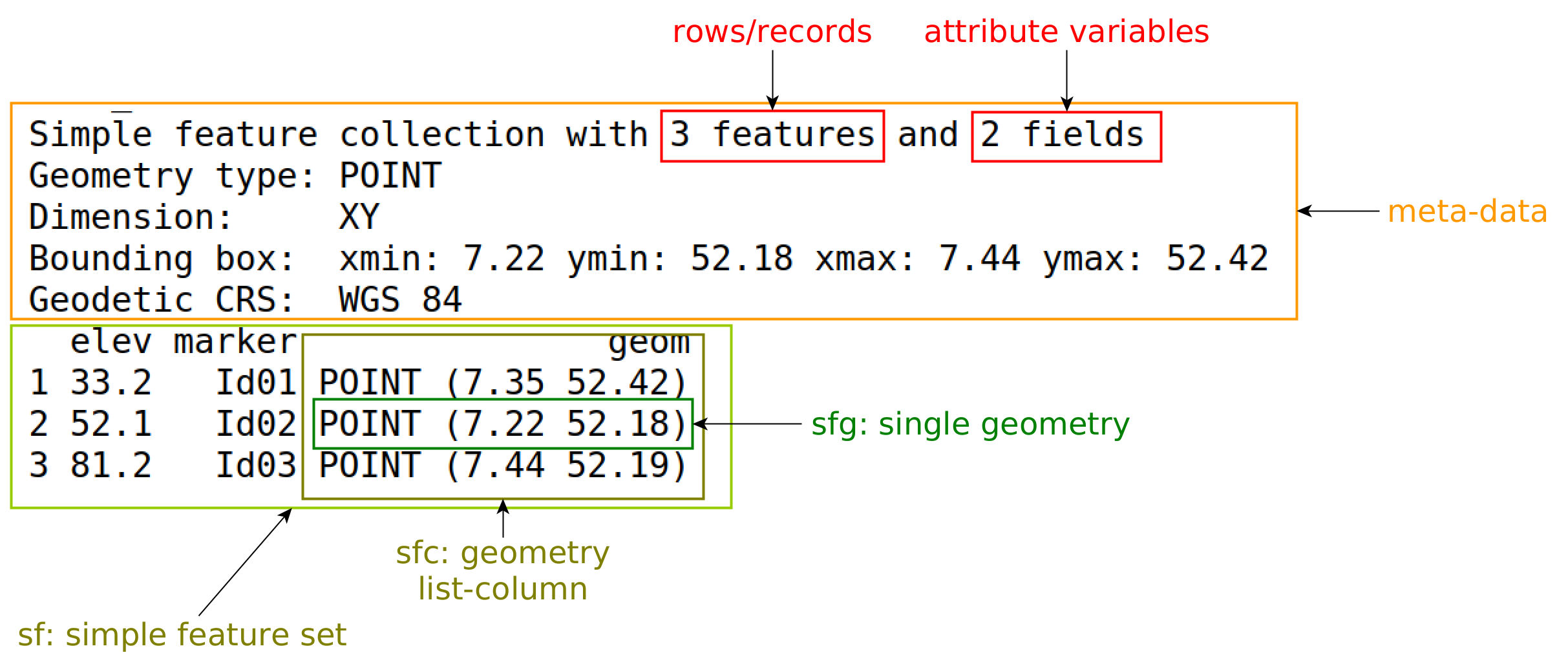
# location coordinates
p1 <- st_point(c(7.35, 52.42))
p2 <- st_point(c(7.22, 52.18))
p3 <- st_point(c(7.44, 52.19))
# geometry column
sfc <- st_sfc(list(p1, p2, p3), crs = 'OGC:CRS84')
# sf class data.frame
st_sf(elev = c(33.2, 52.1, 81.2),
      marker = c("Id01", "Id02", "Id03"), geom = sfc)
# Simple feature collection with 3 features and 2 fields
# Geometry type: POINT
# Dimension:     XY
# Bounding box:  xmin: 7.22 ymin: 52.2 xmax: 7.44 ymax: 52.4
# Geodetic CRS:  WGS 84 (CRS84)
#   elev marker              geom
# 1 33.2   Id01 POINT (7.35 52.4)
# 2 52.1   Id02 POINT (7.22 52.2)
# 3 81.2   Id03 POINT (7.44 52.2)
Functions
tidyverse functions for sf objects
summarizehas 2 extra arguments- do_union (default TRUE) determines whether grouped geometries are unioned on return, so that they form a valid geometry
- is_coverage (default FALSE) in case the geometries grouped form a coverage (do not have overlaps), setting this to
TRUEspeeds up the unioning
st_agr- Gets or sets the “attribute-geometry relationship” (AGR) — that is, how each non-geometry attribute (column) relates to its geometry columnCertain geometric operations — like
st_union,st_intersection, orst_join— may need to know how to handle attributes when geometries are modified or combined.Possible Values
AGR value Meaning Example use “constant” The attribute is constant within the geometry. A country’s name, ISO code, land use, soil type (it doesn’t change across the polygon). “aggregate” The attribute is summed or aggregated when geometries are combined. Population, GDP, or area — if you merge polygons, the attribute should be added. “identity” Identifier An ID or index variable (e.g., grid cell ID). Examples
Single Attribute AGR
# find cells that cross border or don't is_cross_brdr <- st_intersects(grid_de["ID"], st_cast(st_union(shp_de), "MULTILINESTRING"), as_points = FALSE) # subset only cells with 1 (i.e. cross border) sf_grid_de <- st_as_sf(grid_de["ID"], na.rm = FALSE)[lengths(is_cross_brdr) > 0,] attr(sf_grid_de, "agr") #> ID #> <NA> #> Levels: constant aggregate identity st_agr(sf_grd_de) = "identity" attr(sf_grid_de, "agr") #> ID #> identity #> Levels: constant aggregate identity- From Geospatial, Modeling >> Interpolation >> Kriging >> Examples >> Example 3
- There’s only 1 attribute in this sf object, and it’s a cell ID for a grid. Later
st_intersectionis used, so the AGR gets set to “identity.”
Set AGRs for multiple attributes
library(sf)

# Simple example with two attributes
nc <- st_read(system.file("shape/nc.shp", package="sf"), quiet = TRUE)
nc_small <- nc[1:3, c("NAME", "AREA", "geometry")]

# Check AGR
st_agr(nc_small)
#>      NAME      AREA
#>       <NA>       <NA>
#> Levels: constant aggregate identity

st_agr(nc_small) <- c(NAME = "constant", AREA = "aggregate")
st_agr(nc_small)
#>      NAME      AREA
#>  constant aggregate
#> Levels: constant aggregate identity
Measures
Distances
st_crs(sf_obj)$unitstells what unit of measurement is that coordinate system- Planar Distances (Euclidean, feet or meters, projected coordinates)
- If your study area is small (e.g., a city block, a small park), the difference between planar and Great Circle distances will be minimal, and planar distances are usually sufficient
- “For a city-sized area like Chicago, which spans roughly 15 km east-west and 25 km north-south, the distortion from using planar distance with raw lat/lon coordinates would be relatively small. At Chicago’s latitude (approximately 41.8°N), and over such short distances, the error compared to Great Circle distance would typically be less than 1%. errors of several kilometers for distances measured across the state.”
- Uses Planar (projected) Coordinate Systems,
- UTM (Universal Transverse Mercator): Divides the Earth into 60 zones, each 6 degrees of longitude wide. Each zone has its own origin and projection parameters designed to minimize distortion within that zone.
- e.g. UTM Zone 18N
- State Plane Coordinate System: Used in the United States, each state (or sometimes a portion of a state) has its own projection and parameters optimized for that specific area
- UTM (Universal Transverse Mercator): Divides the Earth into 60 zones, each 6 degrees of longitude wide. Each zone has its own origin and projection parameters designed to minimize distortion within that zone.
- Great Circle Distances (latitude, longitude, degrees, geodetic coordinates)
- The shortest distance between two points along a great circle (a circle that divides the sphere into two equal hemispheres). It’s the most accurate for Earth-based calculations.
- If your study area is large (e.g., a state, a country, multiple continents), the Earth’s curvature becomes significant, and you must use Great Circle distances.
- Uses Geographic (angular) Coordinate Systems
- A latitude and longitude system in degrees, which are angles measured on the Earth’s surface. They are inherently spherical (or more accurately, ellipsoidal).
- e.g. WGS 84 (World Geodetic System 1984), a widely used geographic coordinate system based on the WGS 84 ellipsoid with EPSG code 4326
- Spherical Distances (latitude, longitude, km)
- Measured along a small circle parallel to the equator (constant latitude). This is simpler to calculate (euclidean vs trigonometric) than Great Circle distance, but less accurate, especially at high latitudes.
- Unless you’re working with real-time calculations or massive datasets (millions of pairs of points), the computational savings probably wouldn’t justify the trade-off in accuracy.
- Latitude is treated as a straight-line distance rather than accounting for the curvature of the Earth, which is why it’s less accurate than Great Circle distance at high latitudes.
- Measured along a small circle parallel to the equator (constant latitude). This is simpler to calculate (euclidean vs trigonometric) than Great Circle distance, but less accurate, especially at high latitudes.
Points in Polygons
st_centroid- Finds the point in the center of a polygonThis could be in a body of water (i.e. outside the polygon) for some oddly shaped boundaries such as counties with coastal inlets or bays, or gerrymandered districts, etc.
Example
# spherical
NY8_sf <-
  st_read(
    system.file("shapes/NY8_bna_utm18.gpkg",
                package = "spData"),
    quiet = TRUE
  )
NY8_ct_sf <-
  st_centroid(
    st_geometry(NY8_sf),
    of_largest_polygon = TRUE
  )
# planar
st_is_longlat(NY8_ct_sf)
#> [1] FALSE

ny8_crs <- st_crs(NY8_sf)
# Set the CRS of the centroid geometry
NY8_ct_sf_sph <-
  st_set_crs(NY8_ct_sf,
             ny8_crs)
# spherical
st_is_longlat(NY8_ct_sf)
#> [1] TRUE
st_point_the_surface- Guarantees that the point will fall on the surface of a member polygon. (Code is the same asst_centroid)- The point won’t necessarily be near the center.
- Can generate random points in a polygon for labels
Generate a (potentially) more central point guaranteed to be within the polgon
ny8_circs <- st_inscribed_circle(st_geometry(NY8_sf), nQuadSegs = 0) NY8_cic_sf <- st_cast(ny8_circs, to = "POINT")st_inscribed_circle: Calculates the largest circle that can fit entirely within each geometry in NY8_sf.- nQuadSegs controls the number of segments used to approximate the circle. When set to 0, it returns a 2-point LINESTRING (center point and a point on the circle). This representation is more accurate (center + radius) and efficient than using a polygon. This setting is only available for GEOS >= “3.9.0”. In general, a higher value (e.g. default = 30) results in a smoother polygon.
st_cast: Converts the 2-point LINESTRING to just a (center) point (to = “POINT”)
Example: Find counties within 50km from Orange County (source)
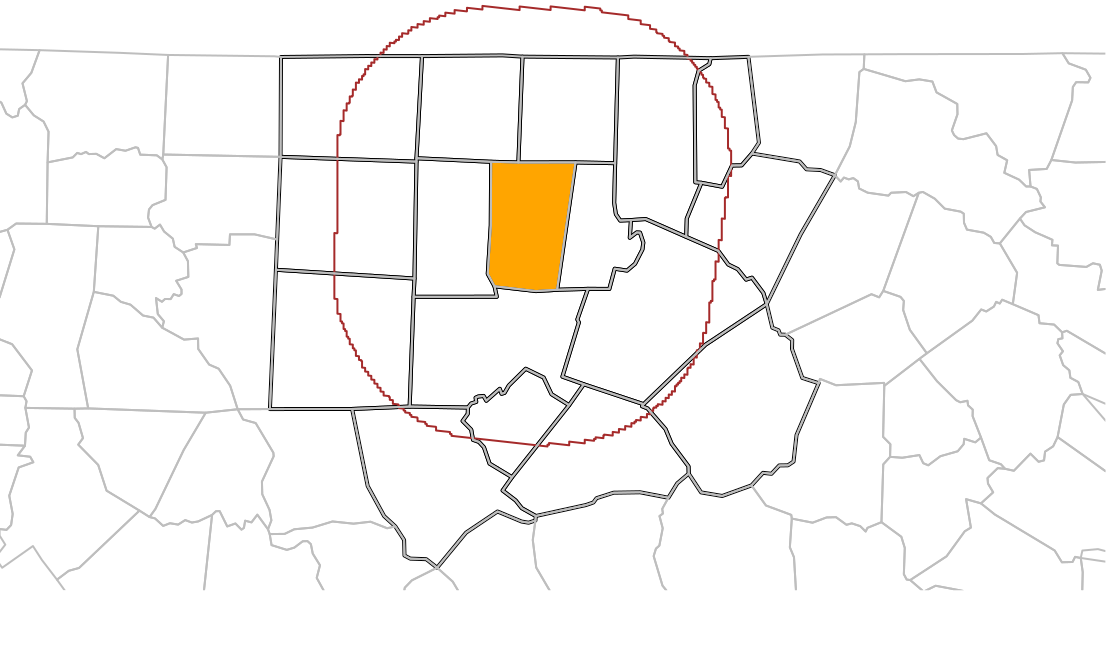
file <- system.file("gpkg/nc.gpkg", package = "sf")
nc <- st_read(file)
# Reading layer `nc.gpkg' from data source
#   `/home/edzer/R/x86_64-pc-linux-gnu-library/4.4/sf/gpkg/nc.gpkg'
#   using driver `GPKG'
# Simple feature collection with 100 features and 14 fields
# Geometry type: MULTIPOLYGON
# Dimension:     XY
# Bounding box:  xmin: -84.3 ymin: 33.9 xmax: -75.5 ymax: 36.6
# Geodetic CRS:  NAD27

orange <- nc |>
  dplyr::filter(NAME == "Orange")

wd <- st_is_within_distance(
  nc,
  orange,
  units::set_units(50, km)
)

# counties within 50km
o50 <- nc |>
  dplyr::filter(lengths(wd) > 0)
nrow(o50)
# [1] 17

# plot
og <- st_geometry(orange)
buf50 <- st_buffer(og, units::set_units(50, km))
all <- c(buf50, st_geometry(o50))

plot(st_geometry(o50), lwd = 2, extent = all)
plot(og, col = 'orange', add = TRUE)
plot(buf50, add = TRUE, col = NA, border = 'brown')
plot(st_geometry(nc), add = TRUE, border = 'grey')
Transformations
Buffer
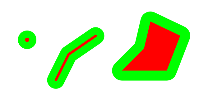
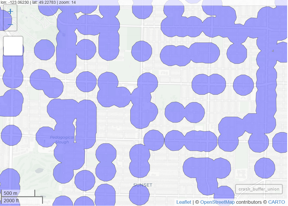
Example: (source)
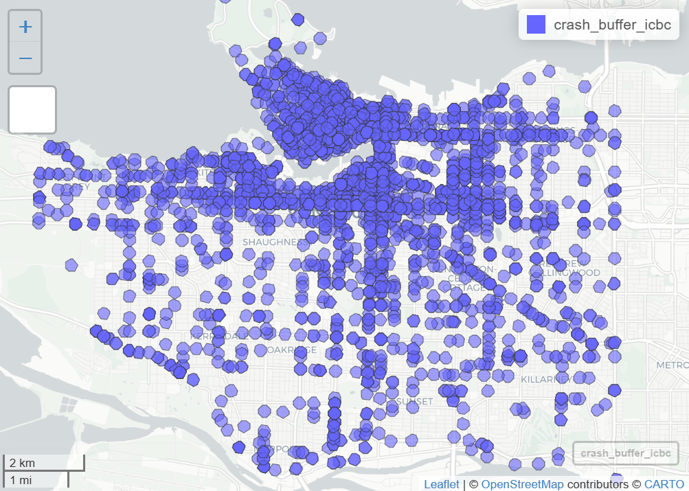
st_crs(icbc_crash_van)$units
#> [1] "m"

crash_buffer_icbc <-
  st_buffer(icbc_crash_van, dist = 150)
mapview(crash_buffer_icbc)

# or

ggplot() +
  geom_sf(icb_crash_van, fill = "lightblue") +
  geom_sf(crash_buffer_icbc, fill = "red")
For geodetic coordinates, dist is specified in meters unless you have
sf_use_s2set to FALSE. In that case, it’s in degrees.For projected coordinates, dist is in the units of those coordinates
Union

[Intersection]{.underline}
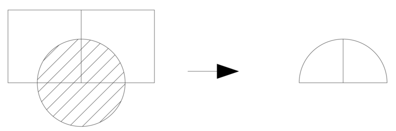
st_intersect- A binary predicate (i.e. logical) that tests whether a geometry/cell in a grid/etc. intersects another geometry/cell in a grid/etc. Outputs 1/0.st_intersection- A geometric processing step that actually computes the intersection shapes.Example:
st_intersection(source)
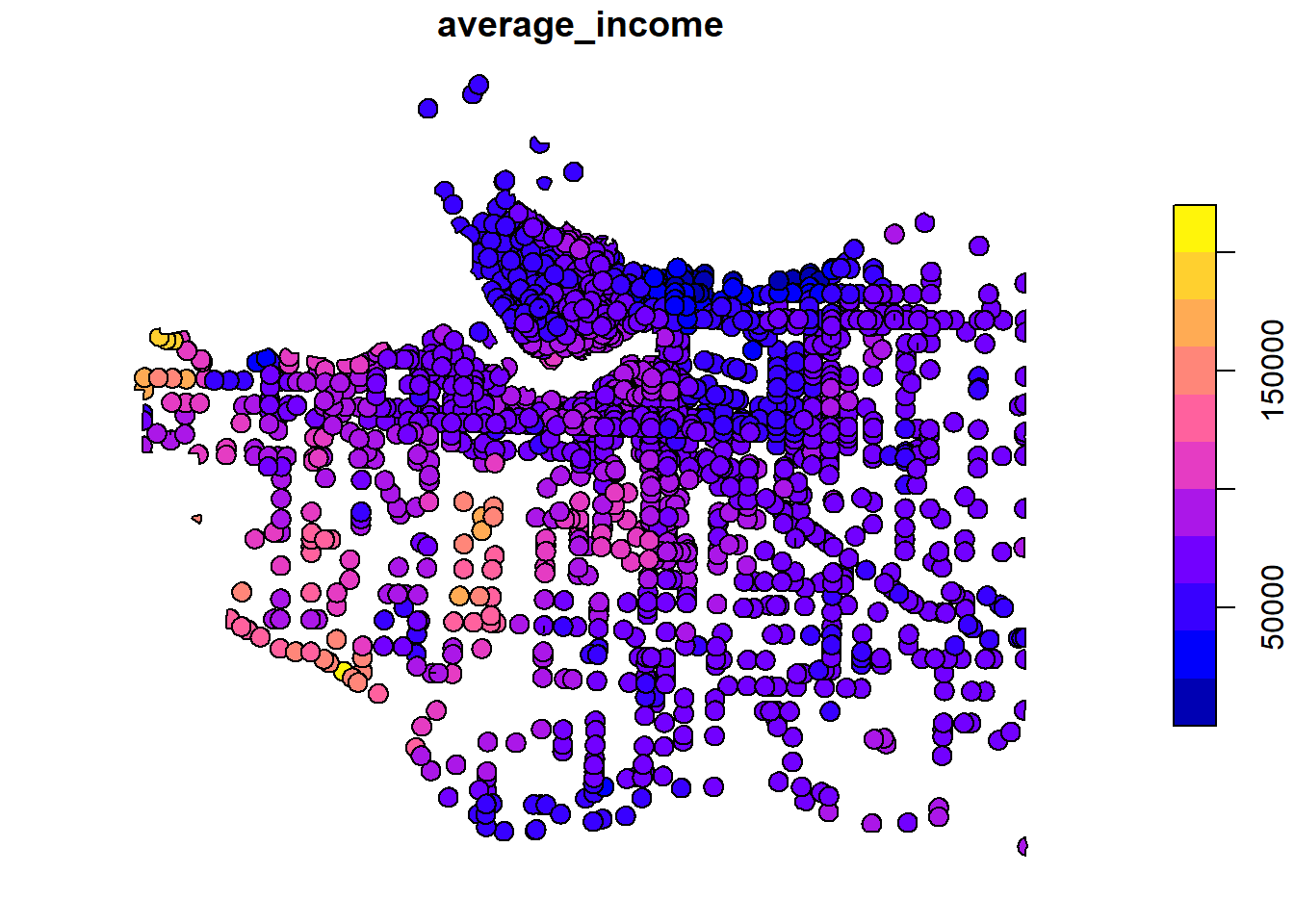
intersect_van_census_crash_buffer <- st_intersection(census_intersects_cntrd, crash_buffer_icbc) average_income_by_crash_buffer <- intersect_van_census_crash_buffer |> group_by(uniqid) |> summarise(average_income = mean(v_CA16_2397, na.rm = TRUE)) plot(average_income_by_crash_buffer["average_income"])Example:
st_intersectsandst_intersection(From Geospatial, Modeling >> Interpolation >> Kriging >> Examples >> Example 3)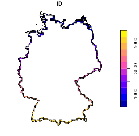
1is_cross_brdr <- st_intersects(grid_de["ID"], st_cast(st_union(shp_de), "MULTILINESTRING"), as_points = FALSE) 2sf_grid_de <- st_as_sf(grid_de["ID"], na.rm = FALSE)[lengths(is_cross_brdr) > 0,] # agr needs set for st_intersection st_agr(sf_grid_de) = "identity" 3grid_cross_brdr <- st_intersection(sf_grid_de, st_union(shp_de)) plot(grid_cross_brdr)- 1
-
st_intersectfinds grid cell IDs that intersect with country border (st_union(shp_de)) - 2
- Subset only cells that cross the border and creates a sf object for them
- 3
-
st_intersectiontakes those border cells and the polygons from the shape file and computes the intesection polygons (I think the colors are possibly referring to the cell IDs?)
Joins
Also see
- Aggregations >> Example 5 >> Area Weighted Aggregation (
st_equals) - Geospatial, Analysis >> Descriptive >> Average Elevation for Areas (
st_intersects)
- Aggregations >> Example 5 >> Area Weighted Aggregation (
Packages
- {fjoin} - {data.table} extension that supports sf/sfc object joins (retains attributes)
A spatial join is similar to a starndard dataframe join, but the criterion to join records is not equality of attributes but a spatial predicate. (e.g. st_intersects, st_equals, etc)
st_intersectsis the default
The concepts of “left”, “right”, “inner”, or “full” joins remain identical to the non-spatial join as the options for handling records that have no spatial match
Example: largest = TRUE (source)
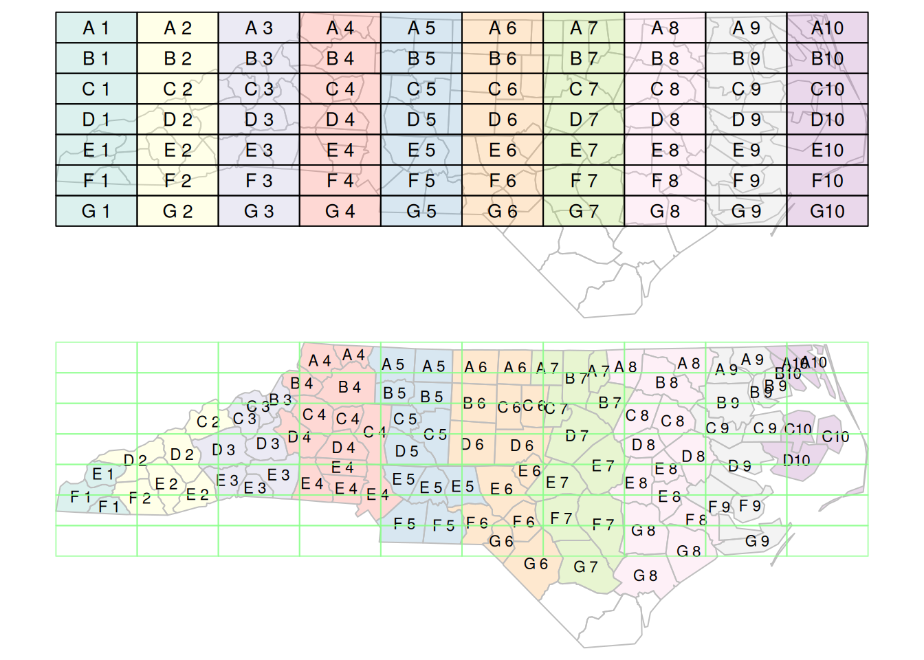
system.file("gpkg/nc.gpkg", package="sf") |> read_sf() |> st_transform('EPSG:2264') -> nc gr <- st_sf( label = apply( expand.grid(1:10, LETTERS[10:1])[,2:1], 1, paste0, collapse = "" ), geom = st_make_grid(nc) ) gr$col <- sf.colors(10, categorical = TRUE, alpha = .3) # cut, to verify that NA's work out: gr <- gr[-(1:30),] suppressWarnings(nc_j <- st_join(nc, gr, largest = TRUE))- The colored grid gets joined to the north carolina polygons and since largest = TRUE, each grid cell gets matched to the polygon (aka record) with the largest overlap
Bounding Boxes
Read only data within a bounding box
Filtering during read can be much faster than “read then filter” if the file has a spatial index
From a URL (source)
# URL to the wind turbine database url <- "/vsizip//vsicurl/https://ftp.cartes.canada.ca/pub/nrcan_rncan/Wind-energy_Energie-eolienne/wind_turbines_database/wind_turbine_database_en.gdb.zip" # List layers in the dataset st_layers(url) # Read and transform the area of interest area_bdd <- read_sf(fs::path("data", "area.geojson")) |> st_transform(crs = st_crs(pts)) # Convert the area geometry to WKT wkt_bdd <- area_bdd |> st_geometry() |> st_as_text() # Read the filtered dataset using the bounding box dat_bdd <- read_sf(url, wkt_filter = wkt_bdd)- Also see Databases, DuckDB >> Extensions >> Geospatial for an example of filter by bounding box through a DuckDB query
From a file (source)
bounds_lonlat <- st_bbox(
  c(xmin = -64.6418,
    xmax = -64.2868,
    ymin = 44.8473,
    ymax = 45.0151),
  crs = st_crs("OGC:CRS84")
)

# Read the CRS of the source
elevation_crs <- st_layers("data/ns-water_elevation.fgb")$crs[[1]]

# Transform the bounds to the CRS of the source
bounds_poly <- bounds_lonlat |>
  st_transform(elevation_crs) |>
  st_as_sfc()

# Read just the data you need
elevation <- st_read(
  "data/ns-water_elevation.fgb",
  wkt_filter = st_as_text(bounds_poly)
)
Aggregations
Misc
- AKA Conservative Region Aggregation or Regridding
- Considers the area of overlap of the source and target geometries, and uses that to weigh the source attribute values into the target value
- Notes from Spatial Data Science, Ch. 5
Methods
- Sub-Areas (\(S_{ij}\)) are the geometries of the original variable values (smaller than Target Areas).
- Target Areas (\(T_{ij}\)) are the new larger geometries that will be the support for the aggregated variable
- Aggregating Extensive Variables
Formula
\[\begin{align} &\hat Y_{j}(T_j)= \sum_{i=1}^p \frac{|A_{ij}|}{|S_i|} Y_i (S_i) \\ &\text{where} \;\; A_{ij} = T_j \cap S_i \end{align}\]
Process
- Calculate intersection area betweem the sub-area (\(S_{i}\)) and the target area (\(T_{j}\)) .
- Calculate the proportion of the intersected area (\(A_{ij}\)) to the sub-area (\(S_{i}\))
- Multiply that proportion (\(|A_{ij}|\;/\;|S_i|\)) times the variable (\(Y_i (S_i)\)) to get the target subarea variable value.
- Repeat for \(p\) sub-areas
- Sum all target subarea variable values to get the target area variable value (\(\hat Y_{j}(T_j)\))
- Aggregating Intensive Variables
The assumption is that the variable has a constant value over each sub-area (\(S_i\)), and therefore has that same value for the intersection with target area (\(T_j\))
Formula
\[\begin{align} &\hat Y_{j}(T_j)= \sum_{i=1}^p \frac{|A_{ij}|}{|T_i|} Y_i (S_i) \\ &\text{where} \;\; A_{ij} = T_j \cap S_i \end{align} \]
- The difference here is the weight is the proportion of the intersection \(A_{ij}\) to the target area (\(T_j\))
Examples
Example: Basic by polygon, by grid cell
# data
dat_no2 <-
  readr::read_csv(system.file("external/no2.csv",
                              package = "gstat"),
                  show_col_types = FALSE)
sf_no2 <-
  st_as_sf(dat_no2,
           crs = "OGC:CRS84",
           coords = c("station_longitude_deg", "station_latitude_deg")) |>
  st_transform(crs)

# shape file with polygons
crs <- st_crs("EPSG:32632")
shp_de <-
  read_sf("https://raw.githubusercontent.com/edzer/sdsr/main/data/de_nuts1.gpkg") |>
  st_transform(crs)

# aggregate by polygon
sf_no2_agg <-
  aggregate(sf_no2["NO2"],
            by = shp_de,
            FUN = mean)
# create grid grid_de <- st_bbox(shp_de) |> # 10km x 10km cells st_as_stars(dx = 10000) |> st_crop(shp_de) # download and clean population data sf_pop <- local({ load(url("https://raw.githubusercontent.com/edzer/sdsr/main/data/ch12.rda"), envir = environment()) get(ls()[1]) }) # aggregate by grid cell grid_agg_pop <- aggregate(sf_pop, st_as_sf(grd, na.rm = FALSE), sum)Example 1: Aggregate extensive variable into quadrants (source)

library(dplyr); library(sf) nc <- read_sf(system.file("gpkg/nc.gpkg", package = "sf")) # create quadrant indicators using two logicals nc$lng <- st_coordinates(st_centroid(st_geometry(nc)))[,1] > -79 nc$lat <- st_coordinates(st_centroid(st_geometry(nc)))[,2] > 35.5 # sum variable by quadrant indicators nc.grp1 <- aggregate(x = nc["SID74"], by = list(nc$lng, nc$lat), FUN = sum) |> (\(d) d[order(d$SID74), ])() # or nc.grp2 <- nc |> group_by(lng, lat) |> summarize(SID74 = sum(SID74)) |> arrange(SID74) nc.grp1["SID74"] |> st_transform('EPSG:32119') |> plot(graticule = TRUE, axes = TRUE)- SID74 is a disease incidence (count) variable
- Counties are grouped by their position (according to the quadrant in which the county centroid is with respect to ellipsoidal coordinate POINT(-79, 35.5)
aggregate’s by argument can also take a shape file object
- If you look at the sf docs for the sf tidyverse functions (See Misc) under the do_union argument, it says, “Using
st_unionresolves internal boundaries, but in case of unioning points, this will likely change the order of the points.”- Therefore, when you compare the output between
aggregateandgroup_by+summarize, the first sets of the points in the geometry column cells will likely be different. That will be because the pairs of points in each polygon are listed in different orders and not because the resulting geometries are different. - In this example, I could not see any difference in the plotted objects whether the union was done via the base R way or the dplyr way.
- Therefore, when you compare the output between
Example 2: Aggregate Multiple Intensive Variables (SDS Ch.16)
This is the Boston housing dataset. NOX is nitrous oxide pollution measurement and NOX_ID is the ID variable for the area where the measurement took place. CHAS is an indicator of whether the tract is close to the Charlestown river.
The variables are at the census tract level and the goal here is to aggregate them to the NOX measurement area using NOX_ID.
In this example I show a couple base R options and a dplyr option Continued in Example 3
pacman::p_load( dplyr, sf, spData ) boston_506 <- sf::st_read(system.file("shapes/boston_tracts.gpkg", package = "spData")[1], quiet = TRUE) boston_506$CHAS <- as.factor(boston_506$CHAS) # just cleaning- The {sf} docs say that {dplyr} needs to be loaded, but if need be, I think you could just use dplyr::function syntax and be fine.
ls_nox_ids <- list(as.character(boston_506$NOX_ID)) 1boston_96 <- aggregate(x = boston_506[, "NOX_ID"], by = ls_nox_ids, FUN = unique) boston_96$NOX <- aggregate(boston_506$NOX, ls_nox_ids, mean)$x boston_96$CHAS <- aggregate(as.integer(boston_506$CHAS)-1, # as.integer makes its values (1,2) ls_nox_ids, max)$x # or 2boston_96_2 <- aggregate(boston_506[, "NOX"], ls_nox_ids, mean) colnames(boston_96_2)[1] <- "NOX_ID" boston_96_2$CHAS <- aggregate(as.integer(boston_96_2$CHAS)-1, # as.integer makes its values (1,2) ls_nox_ids, max)$x # or 3boston_96_d <- boston_506 |> group_by(NOX_ID) |> summarize(NOX = mean(NOX), CHAS = max(as.integer(CHAS) - 1))- 1
- Option 1: The first aggregate call is just to perform the union of the geometries . The next couple aggregate calls aggregate the variables and add them to the first one.
- 2
-
Option 2: Union the geometries and aggregate one of the variables at the same time. aggregate automatically creates a generic grouping variable name which can be replaced with NOX_ID by
colnames - 3
-
Option 3: Use sf’s custom dplyr methods to do everything in a few lines. You could probably get
aggregateto handle multiple functions with a udf having conditionals, but I’m going to let that be for now.
Base Map Comparison
original 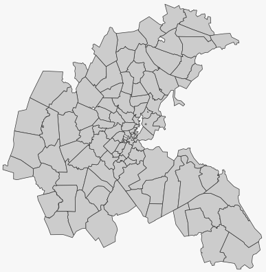
Base R 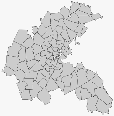
dplyr mapsf::mf_map(boston_506) # origninal data mapsf::mf_map(boston_96) # base r aggregation mapsf::mf_map(boston_96_d) # dplyr aggregation- No differences detected in the unioned geometries
Neighbors Comparison
library(spdep) nb_q_96 <- spdep::poly2nb(boston_96) nb_q_96_d <- spdep::poly2nb(boston_96_d) purrr::map2(nb_q_96, nb_q_96_d, \(x1, x2) all.equal(x1, x2)) |> purrr::list_c() |> (\(x) any(!x))() #> [1] FALSE- Each observation’s vector of neighbors is pairwise compared across neighbors lists. If any pairs are different, then the output would be TRUE. We got a FALSE, so no differences detected.
Neighbors Plots
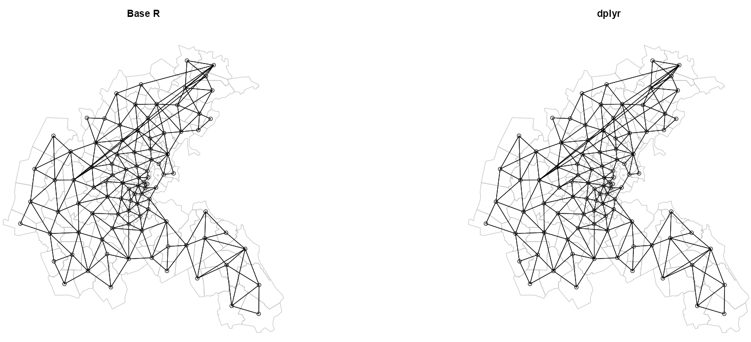
boston_96_ct <- st_centroid(st_geometry(boston_96), of_largest_polygon = TRUE) boston_coords_ct <- st_coordinates(boston_96_ct) boston_96_ct_d <- st_centroid(st_geometry(boston_96_d), of_largest_polygon = TRUE) boston_coords_ct_d <- st_coordinates(boston_96_ct_d) par(mfrow = c(1, 2)) # Base R # plot boundaries plot(st_geometry(boston_96), border = "gray") # plot edges and nodes plot(nb_q_96, coords = boston_coords_ct, add = TRUE) title(main = "Base R") # dplyr plot(st_geometry(boston_96_d), border = "gray") plot(nb_q_96_d, coords = boston_coords_ct_d, add = TRUE) title(main = "dplyr")- The neighbors comparison already told us they were the same, but we can perform a visual inspection just to cement our confidence.
- No differences detected
Example 3: Aggregate Using Weighted Median and Mean (SDS Ch.16)
- Also see Regression, Spatial >> Econometric and Mixed Effects for examples of models using this processed data.
- Continuation from Example 2. If you need to recreate the datesets for the mixed effects models linked to above, then start with example 2 aggregations.
- Response was constructed from counts of ordinal answers to a 1970 census question about house value.
- The response is left- and right-censored in the census source and has been treated as Gaussian.
- The key covariate was created from a calibrated meteorological model showing the annual nitrogen oxides (NOX) level for a smaller number of model output zones (aka Transportation and Air Shed SIMulation model (TASSIM) zones)
- The numbers of houses responding also varies by tract and model output zone.
- There are several other covariates, some measured at the tract level, some by town only, where towns broadly correspond to the air pollution model output zones.
pacman::p_load( dplyr, sf, spData ) boston_506 <- sf::st_read(system.file("shapes/boston_tracts.gpkg", package = "spData")[1], quiet = TRUE) table(boston_506$censored) #> #> left no right #> 2 489 15- Examining the median house values, we find that those for censored values have been assigned as missing, and that 17 tracts are affected
These are explanatory count variables
######## Base R ######## nms <- names(boston_506) ccounts <- 23:31 # aggregate home value cat counts over target geometries (extensive) for (nm in nms[c(22, ccounts, 36)]) { boston_96[[nm]] <- aggregate(boston_506[[nm]], ls_nox_ids, sum)$x } ######## dplyr ######## cols_to_sum <- names(boston_506)[c(22:31, 36)] tib_boston_sums <- boston_506 |> group_by(NOX_ID) |> summarize(across(all_of(cols_to_sum), sum))- 22: units: Number of single family houses
- 23-31:
- cu5k: Count of units under USD 5,000
- c5_7_5: Counts of units from USD 5,000 to 7,500
- C*_*: Other unit value interval counts
- co50k: Count of units over USD 50,000
- 36: POP: Tract population
Uses the (freshly aggregated) home value interval counts as weights and applies them to midpoints in order to get the weighted median home values which is the response variable
####### Base R ######### # midpoint values for the unit value interval classes, e.g. 3.5 is the midpoint of 0 and 5 br2 <- c(3.50, 6.25, 8.75, 12.5, 17.5, 22.5, 30, 42.5, 60) * 1000 counts <- as.data.frame(boston_96)[, nms[ccounts]] calc_wt_median <- function(x) { matrixStats::weightedMedian(x = br2, w = x, interpolate = TRUE) } boston_96$median <- apply(counts, 1, calc_wt_median) is.na(boston_96$median) <- boston_96$median > 50000 summary(boston_96$median) #> Min. 1st Qu. Median Mean 3rd Qu. Max. NA's #> 9009 20417 23523 25263 30073 49496 2 ######## dplyr ######## cols_to_wt_med <- names(boston_506)[23:31] tib_boston_median <- tib_boston_sums |> rowwise() |> mutate(median = matrixStats::weightedMedian(x = br2, w = c_across(cols_to_wt_med), interpolate = TRUE)) |> ungroup() |> mutate(median = ifelse(median > 50000, NA, median))- median: Median home values per geometry (formerly census tract, now NOX measurement area (via NOX_ID))
- interpolate = TRUE says linear interpolation is used to get a consistent estimate of the weighted median.
- In
apply, axis = 1, so this is a rowwise operation - There are two output zones with calculated weighted medians over the upper census question limit of $50,000. Therefore, they are removed them, because they also are affected by not knowing the appropriate value to insert for the top class by value.
- i.e. The censored values are removed as before
Calculate weighted mean over target geometries of intensive variables using census tract population values as observation-level weights inside those target geometries.
Typically you aggregate variables to the target geometries. Then apply target geometry populations as weights to get the weighted mean. The splitting on NOX_ID allows you use census tract populations as weights and calculate the weighted mean per target geometry.
####### Base R ######### POP <- boston_506$POP calc_wt_mean <- function(x) { matrixStats::weightedMean(x = x[,1], w = x[,2]) } for (nm in nms[c(9:11, 14:19, 21, 33)]) { s0 <- split(data.frame(boston_506[[nm]], POP), ls_nox_ids) boston_96[[nm]] <- sapply(s0, calc_wt_mean) } boston_94 <- boston_96[!is.na(boston_96$median),] # only for recreating necessary mod objs for reg-spatial example # nb_q_94 <- spdep::poly2nb(boston_94) # lw_q_94 <- spdep::nb2listw(nb_q_94, style="W") ######## dplyr ######## cols_to_wt_mean <- names(boston_506)[c(9:11, 14:19, 21, 33)] tib_boston_means <- as_tibble(boston_506) |> select(all_of(cols_to_wt_mean), NOX_ID, POP) |> group_by(NOX_ID) |> group_map(~ { .x |> select(cols_to_wt_mean) |> purrr::map(\(col) matrixStats::weightedMean(x = col, w = .x$POP)) |> as_tibble() }) |> purrr::list_rbind()- CRIM: Per capita crime
- ZN: Proportions of residential land zoned for lots over 25000 sq. ft per town (constant for all Boston tracts)
- INDUS: Proportions of non-retail business acres per town (constant for all Boston tracts)
- RM: Average numbers of rooms per dwelling
- AGE: Proportions of owner-occupied units built prior to 1940
- DIS: Weighted distances to five Boston employment centers
- RAD: Index of accessibility to radial highways per town (constant for all Boston tracts)
- TAX: Full-value property-tax rate per USD 10,000 per town (constant for all Boston tracts)
- PTRATIO: Pupil-teacher ratios per town (constant for all Boston tracts)
- BB: Black population proportion
- POP: Tract population
Mixed effects (at least the ones in this example) use variables at lower level of aggregation (census tract), and just group by (varying intercepts) by the higher level (NOX_ID).
While no aggregation is needed for the variables, the spatial process is still being modeled at the NOX measurement area level (NOX_ID). So, the neighbor list/spatial weights object will require unioned geometries at that higher level.
Neighbor graphs that contain subgraphs and nodes with no neighbors can create issues with the model fitting, so those observations (only 2) without neighbors are removed. (Subgraph issue is fixed automatically as well)
Including rownames in the neighbors list/ spatial weights object make out-of-sample prediction possible. The newdata will have rownames which get matched to the “region_id” attribute in the spatial weights object.
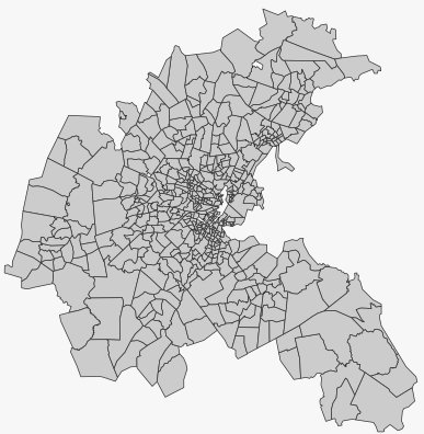
# remove censored values boston_489 <- boston_506[!is.na(boston_506$median),] # only for recreating necessary mod objs for reg-spatial example # nb_q_489 <- spdep::poly2nb(boston_489) # lw_q_489 <- spdep::nb2listw(nb_q_489, style = "W", # zero.policy = TRUE) # get nox_id and its geometries boston_94a <- aggregate(boston_489[,"NOX_ID"], list(boston_489$NOX_ID), unique) nb_q_94a <- spdep::poly2nb(boston_94a) #> Warning in spdep::poly2nb(boston_94a): some observations have no neighbours; #> if this seems unexpected, try increasing the snap argument. #> Warning in spdep::poly2nb(boston_94a): neighbour object has 2 sub-graphs; #> if this sub-graph count seems unexpected, try increasing the snap argument. # find nox_ids with no neighbors NOX_ID_no_neighs <- boston_94a$NOX_ID[which(spdep::card(nb_q_94a) == 0)] # remove nox_ids without neighbors boston_487 <- boston_489[is.na(match(boston_489$NOX_ID, NOX_ID_no_neighs)),] # get new unioned geomtries and create nb list boston_93 <- aggregate(boston_487[, "NOX_ID"], list(ids = boston_487$NOX_ID), unique) row.names(boston_93) <- as.character(boston_93$NOX_ID) # clean, subgraphs have been fixed as well nb_q_93 <- spdep::poly2nb(boston_93, row.names = unique(as.character(boston_93$NOX_ID)))cardcreates a vector of neighbor totals for each NOX_ID
Example 4: Large data may crash R when doing aggregations
Could result in an expensive union operation over identical geometries and a R session crash
Notes from thread (Data with 100K rows crashed R.)
Option 1: Set do_union = FALSE in
summarizetx_income_groups <- get_acs( geography = "tract", table = "B19001", state = "TX", year = 2020, geometry = TRUE ) |> filter(variable != "B19001_001") |> mutate(bracket = case_when( variable > "B19001_012" ~ "Above $100k", TRUE ~ "Below $100k" )) |> group_by(GEOID, bracket) |> summarize(n_households = sum(estimate, na.rm = TRUE), do_union = FALSE)- If you just need the aggregated attribute values and not the geometry union.
Option 2: Perform calculation without geometries then join
tx_income_groups <- get_acs( geography = "tract", table = "B19001", state = "TX", year = 2020, geometry = FALSE ) |> filter(variable != "B19001_001") |> mutate(bracket = case_when( variable > "B19001_012" ~ "Above $100k", TRUE ~ "Below $100k" )) |> group_by(GEOID, bracket) |> summarize(n_households = sum(estimate, na.rm = TRUE)) tx_tracts <- tracts("TX", cb = TRUE, year = 2020) |> select(GEOID) tx_income_groups <- tx_tracts |> left_join(tx_income_groups, by = "GEOID")- {tidycensus} has an arg to bypass d/ling the geometries, geometry = FALSE and a separate
tractsfunction to get the census tract geometries
- {tidycensus} has an arg to bypass d/ling the geometries, geometry = FALSE and a separate
Example 5: From points of 100m cells to 10km cells
- This data and aggregation are part of Geospatial, Modeling >> Interpolation >> Kriging >> Examples >> Example 3
- Also includes the population density calculation
- German population density is used as a predictor for NO2 concentration in air.
- Population data is from a recent census
- The population data file consists of the value and point geometries (even though the data is for a 100m grid cells)
- The goal is to create a population density variable, so the hard part is calculating a reasonably accurate area from square grid cells (i.e. the overlapping parts of the border cells need to be cut off)
- Aggregation to the 10km cell grid is relatively straightforward. No 100m cell grid need be created. The point geometries are evidently enough.
- Aggregation and area-correction are performed by 2 different methods: manually and area-weighted aggregation. Two different area-weighted aggregation workflows are demonstrated: via raster and via polygon.
- tl;dr Although the area-weighted raster method is pretty fast, the manual way is probably fastest (didn’t time it). While the area-weighted method is more accurate and less complicated code-wise, the manual way is probably accurate enough for most use cases.
pacman::p_load( dplyr, ggplot2, sf, stars, gstat ) # no2 data dat_no2 <- readr::read_csv(system.file("external/no2.csv", package = "gstat"), show_col_types = FALSE) crs <- st_crs("EPSG:32632") sf_no2 <- st_as_sf(dat_no2, crs = "OGC:CRS84", coords = c("station_longitude_deg", "station_latitude_deg")) |> st_transform(crs) # germany shape file with polygons shp_de <- read_sf("https://raw.githubusercontent.com/edzer/sdsr/main/data/de_nuts1.gpkg") |> st_transform(crs) # create rectangular grid grid_de <- st_bbox(shp_de) |> # 10km x 10km cells which is a 65 x 87 matrix of 0s st_as_stars(dx = 10000) |> # replaces 0s with NAs for grid cells outside of the border st_crop(shp_de) table(grid_de$values, useNA = "always") #> 0 <NA> #> 3579 2076 # download population data for 100m grid cells. Comes with point geometry sf_pop <- local({ load(url("https://raw.githubusercontent.com/edzer/sdsr/main/data/ch12.rda"), envir = environment()) get(ls()[2]) })- Loads NO2 data, Germany shape file, and population data for 100m grid cells.
- A 10km x 10km grid is created from the shape file
A normal aggregation procedure is performed. Then, border cells have their overlapping parts lopped off. Then, the corrected area is calculated.
Aggregate from 100m to 10km cells
# aggregate by grid cell from 100m x 100m to 10km x 10km grid_agg_pop <- aggregate(sf_pop, st_as_sf(grid_de, na.rm = FALSE), sum)- The population data is aggregated to the 10km cell grid.
Fix Overlapping Border Cells
# create column-wise, cell ID matrix grid_de$ID <- 1:prod(dim(grid_de)) # label border cells is_cross_brdr <- st_intersects(grid_de["ID"], st_cast(st_union(shp_de), "MULTILINESTRING"), as_points = FALSE) # subset border cells from grid sf_grid_de <- st_as_sf(grid_de["ID"], na.rm = FALSE)[lengths(is_cross_brdr) > 0,] st_agr(sf_grid_de) = "identity" # create intersection polygons from border cells grid_cross_brdr <- st_intersection(sf_grid_de, st_union(shp_de))- A grid of square cells will overlap the German border. So to get an accurate area, all cell areas must be within the border. Therefore, we need to chop of the parts of border cells that cross the border.
st_intersectis a binary predictate where a 1 indicates a grid cell that crosses the German border and 0 indicates the cell does not cross the borderst_unioncreates a shape (linestring) that’s just the German country border (no provinces)
- agr needs set for
st_intersection(See Geospatial, Preprocessing >> sf >> Functions >>st_agr) st_intersectioncreates intersection polygons of the German border grid cells (See Geospatial, Preprocessing >> sf >> Transformations >> Intersection >> Example 2) (i.e. parts of cells outside the German border get chopped off)
Calculate Density
# fill (inside-border) area matrix cells with cell area (10km x 10km) grid_de$area <- st_area(grid_de)[[1]] + units::set_units(grid_de$values, m^2) # fill (border) area matrix cells with intersection cell areas grid_de$area[grid_cross_brdr$ID] <- st_area(grid_cross_brdr) # calculate population density grid_de$pop_dens <- grid_agg_pop$Einwohner / grid_de$area # sanity check est_pop <- sum(grid_de$pop_dens * grid_de$area, na.rm = TRUE) # verify est_pop # 80323301 [1] true_pop <- sum(sf_pop$Einwohner, na.rm = TRUE) true_pop # [1] 80324282 # relative error (true_pop - as.numeric(est_pop)) * 100 / true_pop # [1] 0.001221299- Inside Border: First the cell area (10km x 10km) is calcuated and that value is inserted where values are 0 (cells inside the German border) and not NA (outside border)
st_areafills a 65 x 87 matrix with the cell area valueset_unitssets the m2 units attribute to the matrix in grid_de so it can be added to the area matrix.- So now the addition of these two terms results in NA + area = NA; 0 + area = area
- Border: Calculates the intersection border cell areas and assigns those area values to border cell ids in
grid_de$area - This method produces a relative error of around 0.001% which should be good enough for most work.
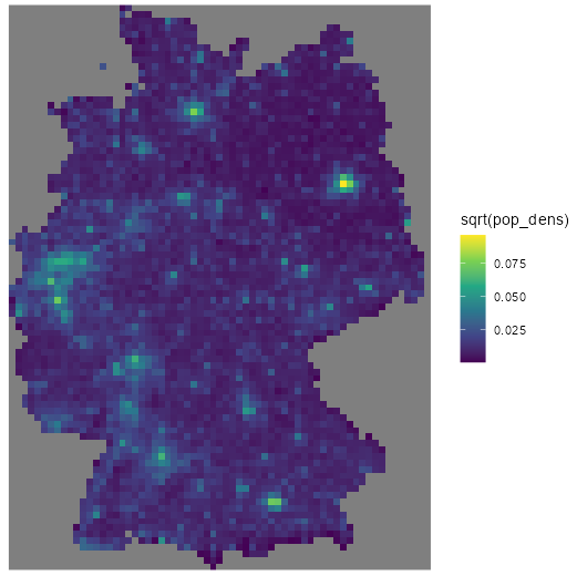
Visualization Code
ggplot() +
  geom_stars(data = grid_de,
             aes(x = x,
                 y = y,
                 fill = sqrt(pop_dens))) +
  scale_fill_viridis_c() +
  coord_equal() +
  theme_void()
Description
- Redistributes the population from the source polygons (100m cells) to the target polygons (10km cells) based on the proportion of overlap. It takes care of the overlapping border problem and aggregation all at once.
- Assumes that the population within a source polygon is uniformly distributed and calculates the geometric intersection between source and target. Then, sums up the proportional values.
- Process
- Calculates precise coverage fractions: For each 100m population raster cell, determine exactly what fraction of that cell falls within each 10km grid polygon. This is done using computational geometry rather than simple point-in-polygon tests.
- Weights values by coverage: Each raster cell’s value (population count) is multiplied by its coverage fraction within the polygon.
- Sums the weighted values: All weighted values are summed to get the total for each 10km grid cell.
- This method produces what’s effectively 100% accuracy, although it’s much more computationally intensive
- The tiny difference (3 people) is likely due to floating-point precision or edge effects at the outer boundary.
{exactextractr} (Raster)
library(exactextractr); library(terra) # Convert to sf polygons grid_sf <- st_as_sf(grid_de, na.rm = FALSE) grid_sf$ID <- seq_len(nrow(grid_sf)) grid_sf_pop <- sf_pop |> st_buffer(dist = 50, endCapStyle = "SQUARE", nQuadSegs = 1) # derive bounding box from grid_sf_pop bb <- st_bbox(grid_sf_pop) # Create 100m raster aligned to pop cells r100 <- rast( xmin = bb["xmin"], xmax = bb["xmax"], ymin = bb["ymin"], ymax = bb["ymax"], resolution = 100, crs = st_crs(grid_sf_pop)$wkt ) pop_r <- rasterize( vect(grid_sf_pop), r100, field = "Einwohner", fun = "sum" ) # should match exactly (aside from floating-point rounding) global(pop_r, "sum", na.rm = TRUE)[1] #> sum #> Einwohner 80324282 sum(grid_sf_pop$Einwohner) #> [1] 80324282 grid_sf$Einwohner <- exact_extract(pop_r, grid_sf, "sum") sum(grid_sf$Einwohner, na.rm = TRUE) #> [1] 80324279 sum(grid_sf_pop$Einwohner, na.rm = TRUE) #> [1] 80324282 # area in km² grid_sf$area_km2 <- units::set_units(st_area(grid_sf), "km^2") |> units::drop_units() grid_sf$pop_dens <- grid_sf$Einwohner / grid_sf$area_km2- This raster method took 138.14 sec (almost entirely by
rasterize) frombboxtoexact_extract
Visualization Code
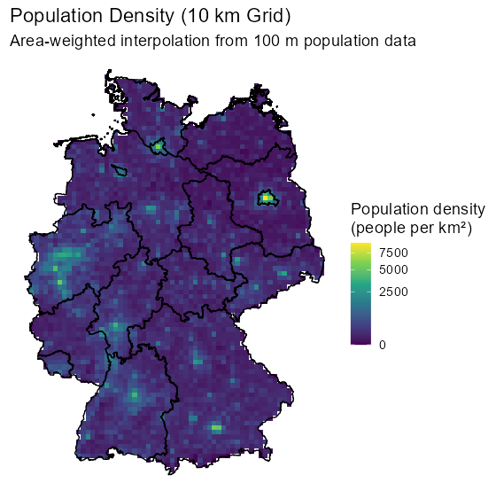
# Assign the calculated density back to the original stars object
# (This works because grid_sf was created from grid_de with na.rm=FALSE, so the cell order matches)
grid_de$pop_dens <- grid_sf$pop_dens
grid_masked <- grid_de[shp_de]

# Plot the stars object directly
ggplot() +
  geom_stars(data = grid_masked,
             aes(fill = pop_dens)) +
  geom_sf(data = shp_de,
          fill = NA,
          color = "black",
          linewidth = 0.5) +
  scale_fill_viridis_c(
    name = "Population density\n(people per km²)",
    trans = "sqrt",
    na.value = "transparent"
  ) +
  coord_sf() +
  theme_void(base_size = 14) +
  labs(
    title = "Population Density (10 km Grid)",
    subtitle = "Area-weighted interpolation from 100 m population data"
  )
{chopin} (Polygon)
library(chopin) # Convert to sf polygons grid_sf <- st_as_sf(grid_de, na.rm = FALSE) grid_sf$ID <- seq_len(nrow(grid_sf)) # 100m cell grid fpr population data grid_sf_pop <- sf_pop |> st_buffer(dist = 50, endCapStyle = "SQUARE", nQuadSegs = 1) # aggregate from 100m to 10km cells aw <- summarize_aw( x = grid_sf, y = grid_sf_pop, target_fields = "Einwohner", id_x = "ID", fun = "sum" ) # sanity check sum(aw$Einwohner, na.rm = TRUE) # [1] 80324279 sum(sf_pop$Einwohner, na.rm = TRUE) # [1] 80324282 # calculate population density per km^2 aw$area <- st_area(aw) aw$pop_density <- aw$Einwohner / (as.numeric(aw$area) / 1e6)- This polygon method took 505.92 sec which was just the
summarize_awfunction - Could also use
st_interpolate_awfrom {sf}, but I had trouble with it. Thissummarize_awfrom {chopin} worked for me more easily.
Visualization Code
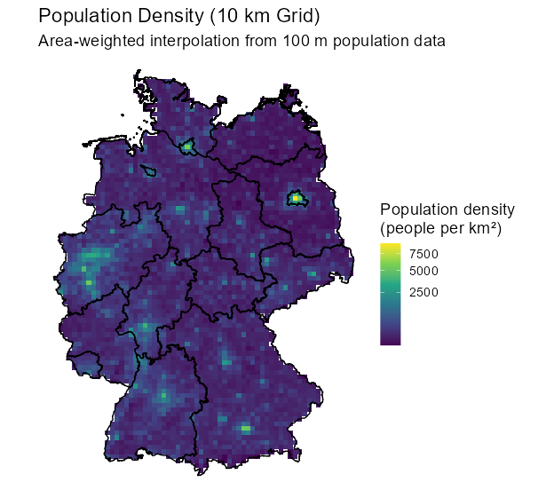
# Since grid_sf was created from grid_de with the same cell order
# Just directly assign where we have matches
grid_sf$pop_dens <- NA_real_

# Use spatial join to match aw back to grid_sf
matched <- st_join(grid_sf, aw, join = st_equals)
grid_sf$pop_dens <- matched$pop_density

# Now assign to stars and mask so only Germany shows
grid_de$pop_dens <- grid_sf$pop_dens
grid_masked <- grid_de[shp_de]

ggplot() +
  geom_stars(data = grid_masked,
             aes(fill = pop_dens)) +
  geom_sf(data = shp_de,
          fill = NA,
          color = "black",
          linewidth = 0.5) +
  scale_fill_viridis_c(
    name = "Population density\n(people per km²)",
    trans = "sqrt",
    na.value = "transparent"
  ) +
  coord_sf() +
  theme_void(base_size = 14) +
  labs(
    title = "Population Density (10 km Grid)",
    subtitle = "Area-weighted interpolation from 100 m population data"
  )
Example 6: Mean across regions per day; {stars} (source)
Code
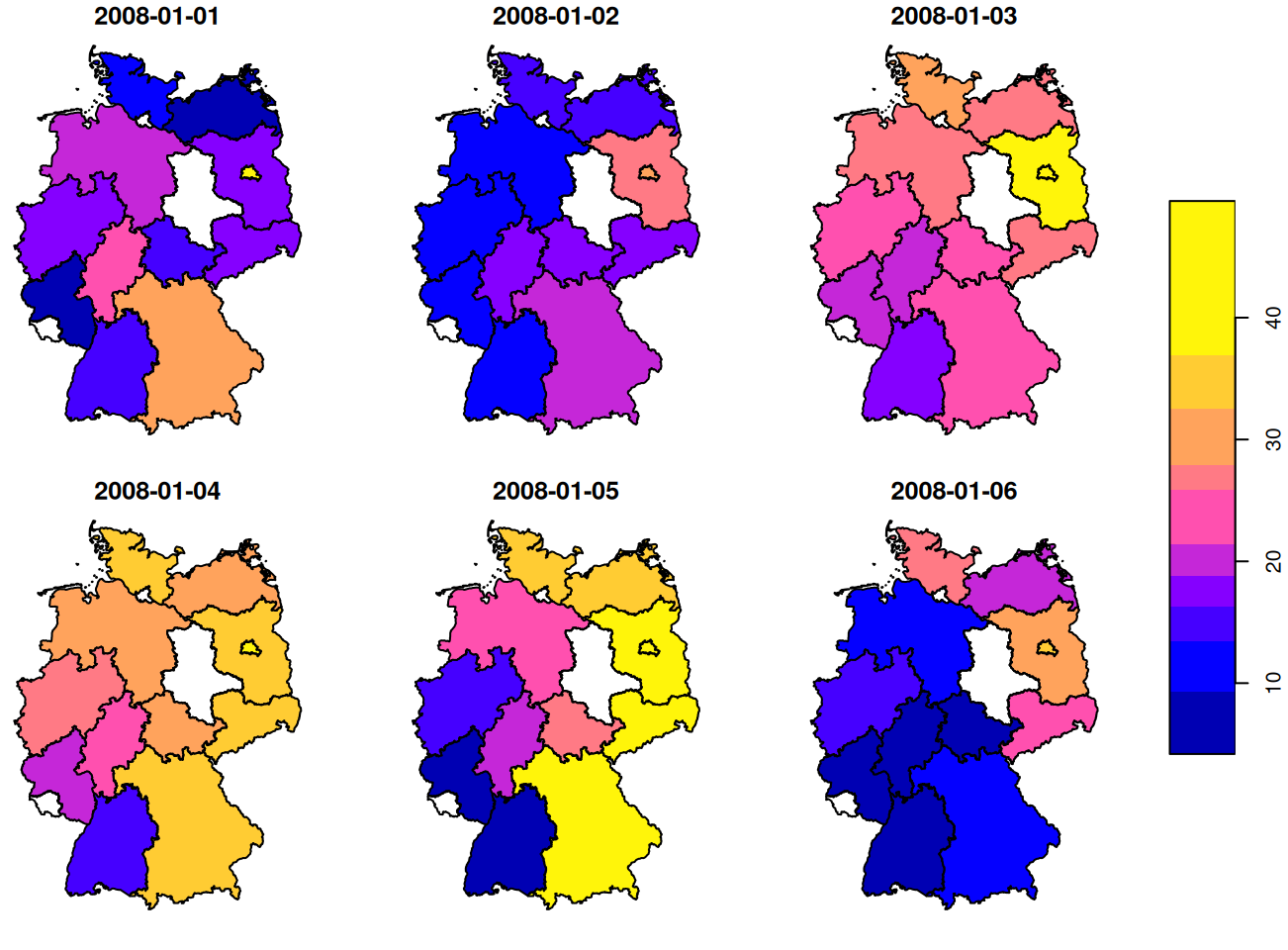
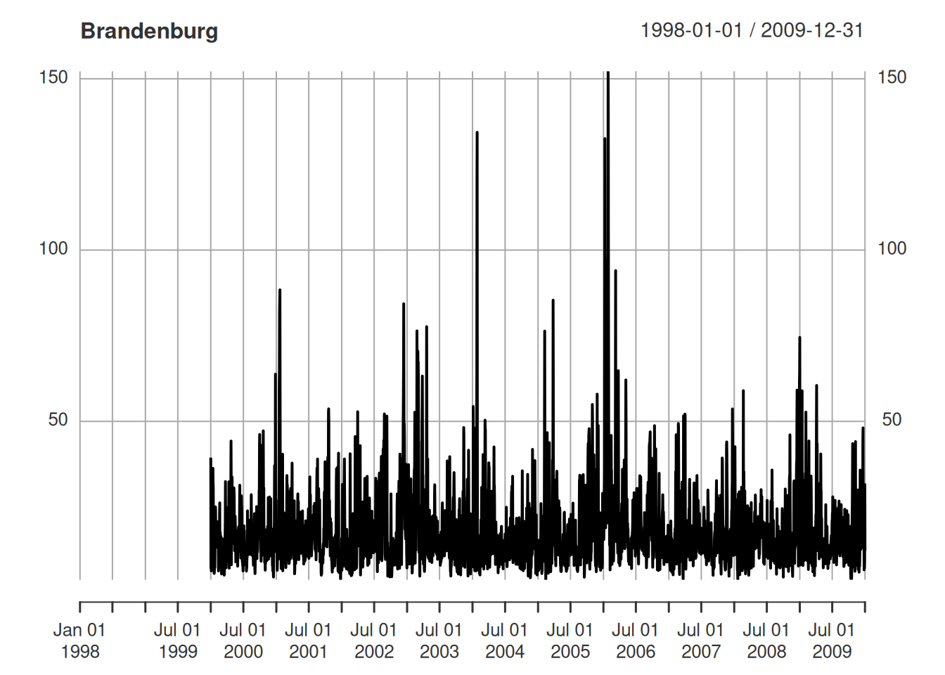
library(dplyr); library(stars) # convert to space x time matrix to stars data(air, package = "spacetime") sfc_stations <- stations |> sf::st_as_sf(coords = c("coords.x1", "coords.x2"), crs = 4326) |> sf::st_geometry() star_dims <- st_dimensions( station = sfc_stations, time = dates ) star_air <- st_as_stars( .x = list(pm10 = air), dimensions = star_dims ) # aggregate and map (star_reg_mean_pm10 <- aggregate( star_air, DE_NUTS1, # germany's provincial polygons; loads alongs w/air mean, na.rm = TRUE )) # stars object with 2 dimensions and 1 attribute # attribute(s): # Min. 1st Qu. Median Mean 3rd Qu. Max. NA's # PM10 1.08 10.9 15.3 17.9 21.8 172 25679 # dimension(s): # from to offset delta refsys point # geom 1 16 NA NA WGS 84 FALSE # time 1 4383 1998-01-01 1 days Date FALSE # values # geom MULTIPOLYGON (...,...,MULTIPOLYGON (... # time NULL star_reg_mean_pm10 |> filter(time >= "2008-01-01", time < "2008-01-07") |> plot(key.pos = 4) # brandenburg xts::as.xts(star_reg_mean_pm10)[,4] |> plot(main = de_nuts1$NAME_1[4])- For details on the conversion from matrix to {stars} object, see Geospatial, Spatio-Temporal >> Data Formats >> Time-wide >> Example 2
- Since this is a {stars} object and time is a dimension along with space (geom), it also is a grouping variable. So we get means for polygons per day.