Multivariate time series analysis seeks to analyze several time series jointly. The rationale behind this is the possible presence of interdependences between the different time series.
Robust to cross-sectional dependence through common factor extraction using principal components.
Provides both group-mean (DHg) and panel (DHp) test statistics with automatic factor number selection via information criteria
Vector Autoregression (VAR)
{bayesianVARs} (Papers) - Efficient Markov Chain Monte Carlo (MCMC) algorithms for the fully Bayesian estimation of vectorautoregressions (VARs) featuring stochastic volatility (SV)
{bvars} - Provides fast and efficient procedures for Bayesian estimation and forecasting using state-of-the-art Vector Autoregressions
{bsvars} - Structural Vector Autoregressions including homo-, heteroskedastic, and non-normal specifications
{bsvarSIGNs} - Structural Vector Autoregressions identified by sign, zero, and narrative restrictions
{micvar} - Implements order selection for Vector Autoregressive (VAR) models using the Mean Square Information Criterion (MIC).
Unlike standard methods such as AIC and BIC, MIC is likelihood-free. This method consistently estimates VAR order and has robust performance under model misspecification
{NetVAR} - VAR Models with tailored regularization structures are provided to uncover network type structures in the data, such as influential time series (influencers).
Full service: handles seasonality, lag selection, granger causality, long run variance, etc.
{statioVAR} - Trend Removal for Vector Autoregressive Workflows
{VARcpDetectOnline} - Sequential Change Point Detection for High-Dimensional VAR Models. Effectively identifies shifts in temporal and cross-correlations within high-dimensional time series data
General
{l1rotation} - Identify Loading Vectors under Sparsity in Factor Models
Uses a sparse representation to overcome rotational indeterminacy and to be able find the true interpretation of how the factors and variables are related.
Constructs State-Space models that can include highly flexible nonlinear predictor effects for both process and observation components by leveraging functionalities from the impressive brms and mgcv packages
{wqrr} - A comprehensive toolbox for wavelet-domain quantile analyses of bivariate and multivariate time series.
Provides Wavelet Quantile Regression and Multivariate Wavelet Quantile Regression, Wavelet Quantile-on-Quantile regression with bootstrap p-values.
The common component is modelled by a static factor model, which allows for strong cross-sectional dependence, whilst a network vector autoregressive process captures the residual co-movements due to the idiosyncratic component
A two-step procedure: the static factors are estimated via principal component analysis, followed by estimation of the network VAR parameters
Applications demonstrated: daily returns, intraday returns, and FRED-MD macroeconomic variables
Examples
US GDP data, S&P 500 data, and oil prices
Mortgage applications, interest rate data, and unemployment rates
Order flow data, price levels, and volatilities
Models
Vector Autoregression (VAR)
Types
Structural: Interdependent time series affect each other contemporaneously
Reduced: Interdependent time series do not affect each other contemporaneously (method commonly used)
Assumes stationarity
VECM (Vector Error Correction Model)
Does not rely on stationarity
Assumes cointegration
Exponentially Weighted Moving Average (EWMA)
BEKK(p, q)
(after Baba, Engle, Kraft, and Kroner) is a multivariate extension of the GARCH
Can maintain the original data representation in the form of matrix.
Reduces the amount of parameters in autoregressive models.
For example, if we use VAR to explore such data, we would have (mn)² parameters in the coefficient matrix. But using MAR, we only have _m_²+_n_². This can avoid the over-parameterization issue in VAR for handling high-dimensional data.
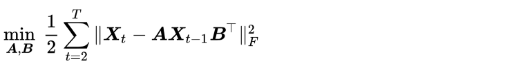
Loss function
Matrices A and B are coefficient matrices than need to be estimated
There are closed form solutions for A and B but the solution to A is dependent on the solution to B and vice versa
The Alternating Least Squares (ALS) Algorithm is used to solve this problem
Dynamic Factor Models (DFM)
Common dynamics of a large number of time series variables stem from a relatively small number of unobserved (or latent) factors, which in turn evolve over time.
For some macroeconomic applications it might be interesting to see whether a set of obserable variables depends on common drivers (unobserved factors). The estimation of such common factors can be done using so-called factor analytical models.
Factor Analysis but for time series
For large sets of time series, which show, in most cases, strong correlation patterns
tl;dr:
Run PCA on bunch of time series that are relevant to the outcome variable you want to model or forecast.
Determine the number of factors (components) from the PCA
Use VAR to determine the number of lags (or potentially leads) for the factors
Fit a model for the outcome variable using the factors and their lags as predictors.
Imports {collapse} and {Rcpp} so it should be very fast
3 methods available
A two-step estimator based on Kalman filtering
fast, and forcasts should be similar to the other 2
A quasi-maximum likelihood approach
Maximum likelihood estimation of factor models on datasets with arbitrary pattern of missing data
{nowcasting}- fit dynamic factor models specific to mixed-frequency nowcasting applications.
The latter two packages additionally support blocking of variables into different groups for which factors are to be estimated, and EM adjustments for variables at different frequencies
{bvartools}
{FARS} - Models and forecasts economic scenarios based on multi-level dynamic factor model
e.g. IoT devices, telecommunication, industrial manufacturing, electric grid
Finance
Macroeconomics
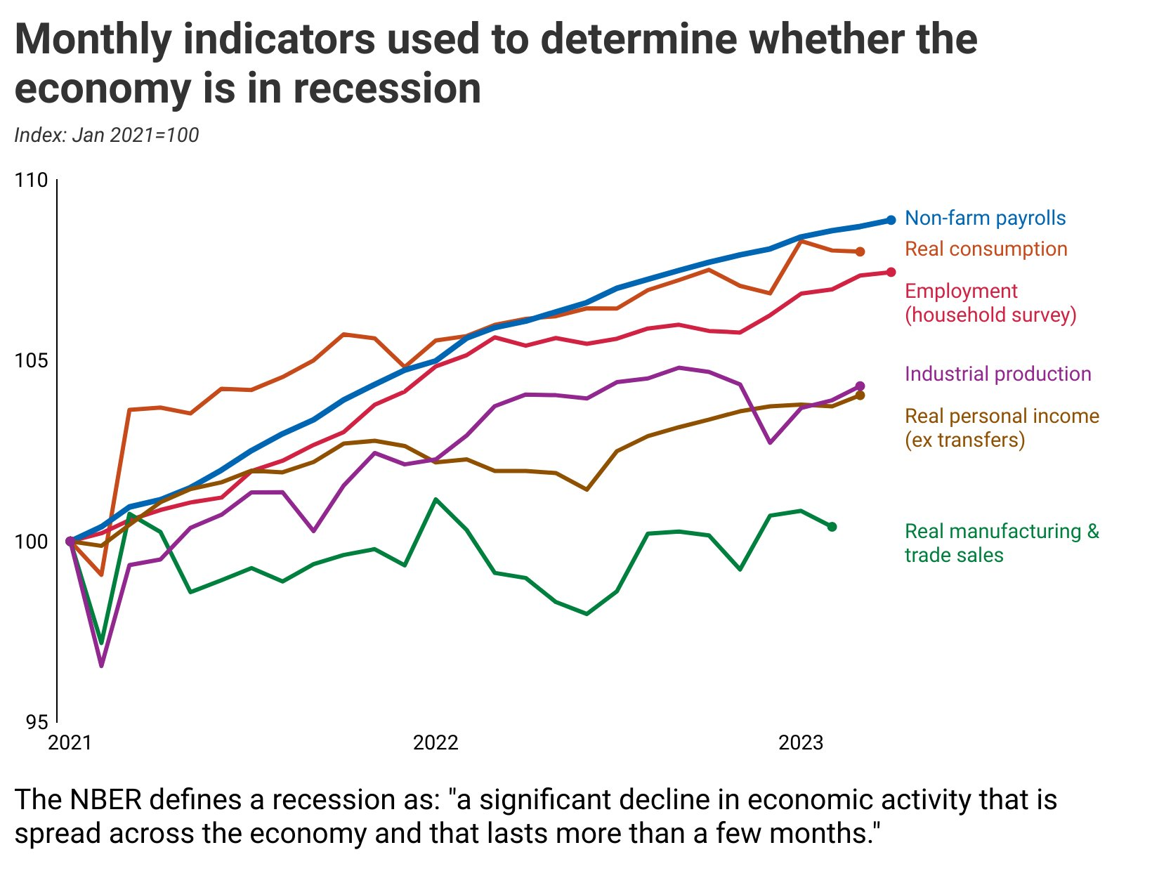
Example: (ebook ch8. introduction): a single-factor DFM fit using 58 quarterly US real activity variables (sectoral industrial production (IP), sectoral employment, sales, and National Income and Product Account (NIPA) series) is used to backcast four-quarter growth rates of four measures of aggregate economic activity (real Gross Domestic Product (GDP), total nonfarm, employment, IP, and manufacturing and trade sales)
Black solid line is the the observed; Red dotted line is the fitted value
Fitted line from lm(outcome ~ factor)
outcome is total nonfarm, employment, IP, or manufacturing and trade sales
factor is from the dfm
R2s of the fits range from 0.73 for GDP to 0.92 for employment.
Chicago Fed fits a factor model called the “cfnai” on these key economic indicators (Thread)
“Structural DFMs, FAVARs, and SVARs are a unified suite of tools with fundamentally similar structures that differ in whether the factors are treated as observed or unobserved. By using a large number of variables and treating the factors as unobserved, DFMs”average out” the measurement error in individual time series, and thereby improve the ability to span the common macroeconomic structural shocks.”
Factor Analytical Model General Form (Static)
xt = λ*ft + ut where ut ∼ N(0,R)
xt is an M-dimensional vector of observable variables
ft is an N×1 vector of unobserved factors
λ is an M×N matrix of factor loadings
ut is an error term
R is a M×M measurement (observation) covariance matrix and assumed to be diagonal
Also known as the measurement equation, which describes the relationship between the observed variables and the factors
Allowing ft to take autocorrelation into account makes it “dynamic”
ft = A1*ft−1 + … + Ap*ft−p + vt where vt∼ N(0,Q)
Ai is the N×N coefficient matrix correponding to the ith lag of factor, f
vt is an error term
Q is the N×N state covariance matrix
Also known as the transition equation, which describes the intertemporal relationships between the factors
Preprocessing
All series must be stationary with no cointegration
All series must be scaled and centered
The number of factors must be chosen.
Then, the number of lags can chosen given the number of factors
Data at different frequencies
{dfms} has a couple methods that approximate values
Duplicate the longer frequency series multiple times. (see article)
e.g. duplicate a quarterly series 3 times in a dataset with monthly time series.
When these series get converted to shorter frequencies before fitting (e.g. quarterly to monthly), the missing values will just be NAs which will cause these series to have less weight in the estimation process. By duplicating them, it gives there values more weight.
If you decide to give these series more weight, you should be relatively certain they’re important to the forecast.
Estimate different factor models for monthly and quarterly series, and combine them for the final prediction (e.g. by aggregating or blocking the monthly factor estimates (?)).
{nowcasting} and {nowcastDFM} provide elaborate models for mixed-frequency nowcasting (but will be slower)
Forecasts
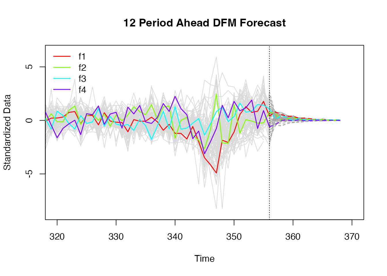
Factors are dynamically forecasted using the transition equation.
The factor forecasts can then be fed to the observation equation to obtain forecasts for the input series
4 factors have been chosen and they’re highlighted
Input series are in gray
Forecasts (after dotted vertical) converge the mean.
quarterly variables, such as US GDP, to be forecast using a large set of monthly variables released with different lags
reduce the information contained in dozens of monthly time series into only two dynamic factors. These two estimated factors, which are initially monthly, are then transformed into quarterly factors and used in a regression against GDP
Backcasting refers to forecasting the value of a yet unpublished variable for a past period, while nowcasting will be with respect to the current period
The chosen number of factors, r∗ will correspond the IC with the lowest value. The penalty in equation IC2 is highest when considering finite sample
Given a strategy to identify one or more structural shocks, a structural DFM can be used to estimate responses to these structural shocks.
description of the error terms to the equations
mean-zero idiosyncratic component et (measurement eq)
idiosyncratic disturbance can be serially correlated. if so, then model is incompletely specified. Solution is to model it as an autoregression
If there is no autocorrelation in the error terms (*unreasonable assumption across most applications), then the model is an exact DFM, and the correlation of one series with another occurs only through the
latent factors
ηt is the q x 1 vector of (serially uncorrelated) mean-zero innovations to the factors (transition eq)
If some of the variables are cointegrated, then transforming them to first differences loses potentially important information that would be present in the error correctionterms (that is, the residual from a cointegrating equation, possibly with cointegrating coefficients imposed). Here we discuss two different treatments of cointegrated variables, both of which are used in the empirical application of Sections 6 and 7.
Option 1: Include the first difference of some of the variables and error correction terms for the others. This is appropriate if the error correction term potentially contains important information that would be useful in estimating one or more factors.
Option 2: include all the variables in first differences and not to include any spreads. Appropriate if the first differences of the factors are informative for the common trend but the cointegrating residuals do not load on common factors
Didn’t understand it lol (pg 427). Think there’s an example in sect 7.2 that will illustrate it.
Example: While there is empirical evidence that these oil prices, for example Brent and WTI, are cointegrated, there is no a priori reason to believe that the WTI-Brent spread is informative about broad macro factors, and rather that spread reflects details of oil markets, transient transportation and storage disruptions, and so forth.
Option 3: specify the DFM in levels or log levels of some or all of the variables, then to estimate cointegrating relations and common stochastic trends as part of estimating the DFM. This approach goes beyond the coverage of this chapter, which assumes that variables have been transformed to be I(0) and trendless.
Banerjee and Marcellino (2009)and Banerjee et al. (2014, 2016) develop a factor-augmented error correction model (FECM) in which the levels of a subset of the variables are expressed as cointegrated with the common factors. The discussion in this chapter about applications and identification extends to the FECM.
The error in estimation of the factors during PCA can be ignored when they are used as regressors
.png)