{modeltuning} - Provides a lightweight framework for model selection and hyperparameter tuning in R.
Offers intuitive tools for grid search, cross-validation, and combined grid search with cross-validation that work seamlessly with virtually any modeling package.
Vignette on scaling with {paws} and an EC2 instance
Algorithms: Grid Search, Random Search, Tree-structured Parzen Estimator, CMA-ES, Gaussian process-based, Algorithm to enable partial fixed parameters, Nondominated Sorting Genetic Algorithm II, A Quasi Monte Carlo sampling
Parallelized by using PostgreSQL or MySQL to communicate between workers
Algorithms: Random Search, Tree of Parzen Estimators (TPE), Adaptive TPE
Parallelized through Spark or MongoDB to communicate between workers
Tree Parameter Categories (many overlap)
Tree Structure and Learning
Training Speed
Accuracy
Overfitting
When the search space is quite large, try the particle swarm method or genetic algorithm for optimization.
Early Stopping can lower computational costs and decrease practitioner downtime
Pairwise Tuning
Tunes a pair of parameters at a time. Once the first pair of parameters is tuned, those values replace the default parameter values, and the next pair of parameters is tuned, etc.
Limits the computational cost of performing a full grid search jointly with all parameters at once supposedly without sacrificing much in terms of predictive performance.
A full grid search or other tuning method can be applied to each pair.
Might be beneficial to create pairs that affect the same tuning area of the model fit (e.g. subsampling, regularization, tree complexity) so that the tuning process might capture any interaction effects between the parameters.
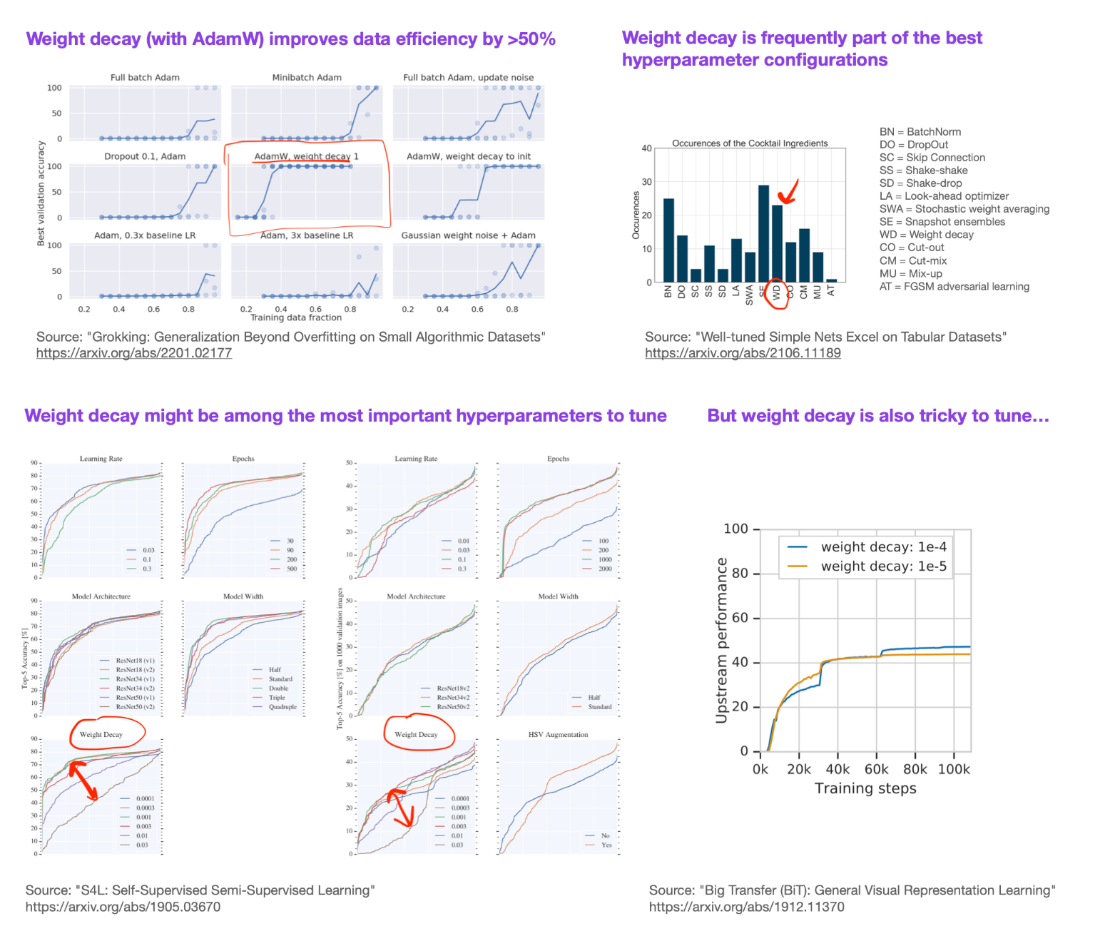
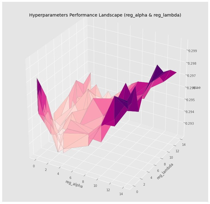
Tuned values for max_depth and eta replace their default values
subsample and colsample_bytree are tuning using the model with the tuned values for max_depth and eta
etc.
Viz
Each pair of parameters along with the loss metric are plotted in a 3D chart
matplotlib::plot_trisurf() uses Surface Triangulation is used to interpolate the gaps between the tested parameter values
If the chart has multiple pronounced dips and bumps (left chart):
May indicate that there’s a minima in one of the dips that might be better than the chosen parameter values as the interpolation process might have smoothed over that area a bit.
Might want to play with the smoothing parameter a bit to try and get a clearer idea of the range of values to further investigate.
Indicates the model is sensitive to this pair of parameters which might translate into a model instability, when we pass a new type of dataset into the tuned model in the deployment domain.
Bayesian Optimization
Packages
{tune::tune_bayes} - tidymodels bayesian optimization; uses a Gaussian process (GP) model; parallelized through {future}
{mlr3mbo} - mlr3 modular implementation for single- and multi-objective Bayesian Optimization
Gaussian processes for low to medium dimensional numeric search spaces and random forests for higher dimensional mixed (and/or hierarchical) search spaces (source)
{rBayesianOptimization} - A Pure R implementation of Bayesian Global Optimization with Gaussian Processes.
Solve Combined Algorithm/Classifier Selection and Hyperparameter optimization (CASH) problem using multiple GP surrogates.
GP surrogates shown to outperform tree-structured Parze estimators (TPE), and TPE is designed to be sequential in nature, thus suffers performance loss in parallel search.
tl;dr
Builds a surrogate model using Gaussian Processes that estimates model score
This surrogate is then provided with configurations picked randomly, and the one that gives the best score is kept for training
Each new training updates the posterior knowledge of the surrogate model.
Components:
The black box function to optimize: f(x).
We want to find the value of x which globally optimizes f(x) (aka objective function, the target function, or the loss function)
The acquisition function: a(x)
Used to generate new values of x for evaluation with f(x).
a(x) internally relies on a Gaussian process model m(X, y) to generate new values of x.
Steps:
Define the black box function f(x), the acquisition function a(x) and the search space of the parameter x.
Generate some initial values of x randomly, and measure the corresponding outputs from f(x).
Fit a Gaussian process model m(X, y) onto X = x and y = f(x) (i.e. surrogate model for f(x))
The acquisition function a(x) then uses m(X, y) to generate new values of x as follows:
Use m(X, y) to predict how f(x) varies with x.
The value of x which leads to the largest predicted value in m(X, y) is then suggested as the next sample of x to evaluate with f(x).
Repeat the optimization process in steps 3 and 4 until we finally get a value of x that leads to the global optimum of f(x).
All historical values of x and f(x) should be used to train the Gaussian process model m(X, y) in the next iteration — as the number of data points increases, m(X, y) becomes better at predicting the optimum of f(x).
Typically outperforms basic bayesian optimization, but the main selling point is it handles complex hyperparameter relationships via a tree structure.
Supports categorical variables (cat hyperparams?) which traditional Bayesian optimization does not.
Process
Train a model with several sets of randomly-selected hyperparameters, returning objective function values.
Split our observed objective function values into “good” and “bad” groups, according to some threshold gamma (γ).
Calculate the “promisingness” score, which is just P(x|good) / P(x|bad).
Determine the hyperparameters that maximize promisingness via mixture models.
Fit our model using the hyperparameters from step 4.
Repeat steps 2–5 until a stopping criteria.
Tips/Tricks
HyperOpt is parallelizable via both Apache Spark and MongoDB. If you’re working with multiple cores, wether it be in the cloud or on your local machine, this can dramatically reduce runtime.
If you’re parallelizing the tuning process via Apache Spark, use a SparkTrialsobject for single node ML models (sklearn) and a Trails object for parallelized ML models (MLlib).
MLflow easily integrates with HyperOpt.
Don’t narrow down the search space too early. Some combinations of hyperparameters may be surprisingly effective.
Defining the search space can be tricky, especially if you don’t know the functional form of your hyperparameters. However, from personal experience TPE is pretty robust to misspecification of those functional forms.
Choosing a good objective function goes a long way. In most cases, error is not created equal. If a certain type of error is more problematic, make sure to build that logic into to your function.
Minimum Impurity Decrease: Sets the threshold for the amount of impurity decrease that must occur in order for there to be another split
Too low may lead to overfit
Too high may lead to underfit
Maximum Features: Randomly choosing a set of features for each split
Useful for high dimension datasets; adds some randomness
Too high can lead to long training times
Too low may lead to underfit
Complexity Parameter (cp): The threshold complexity parameter for {rpart}. The main role of this parameter is to save computing time by pruning off splits that are obviously not worthwhile \[
R_{cp}(T) = R(T) + \text{cp} \cdot |T| \cdot R_1(T)
\]
\(R\) is the risk (?)
\(T_1\) is the tree with no splits
\(|T|\) is the number of splits
cp = 1 will always result in a tree with no splits
For regression models, the scaled cp has a very direct interpretation: if any split does not increase the overall R2 of the model by at least cp then that split is decreed to be, a priori, not worth pursuing.
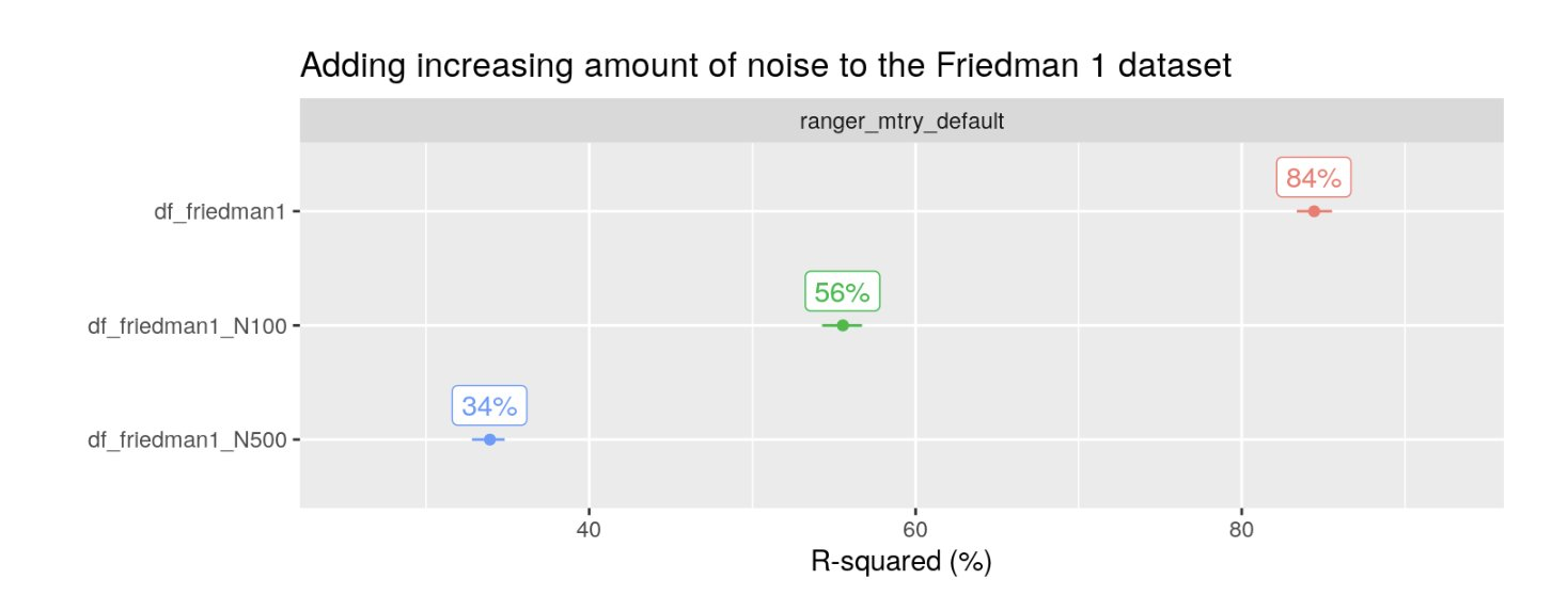
Implicit features selection is performed by splitting, but performance decreases substantially if over 100 noise-like features are added & drastically if over 500 noise-like features
Hyperparameters
num_trees: Total number of trees
This should not be tuned as more trees almost always leads to better performance, but instead should be set the maximum that is computationally practical with your resources and your time constraint (paper which references this paper)
Default: 500 (Ranger) with 2000 potentially a maximum (?)
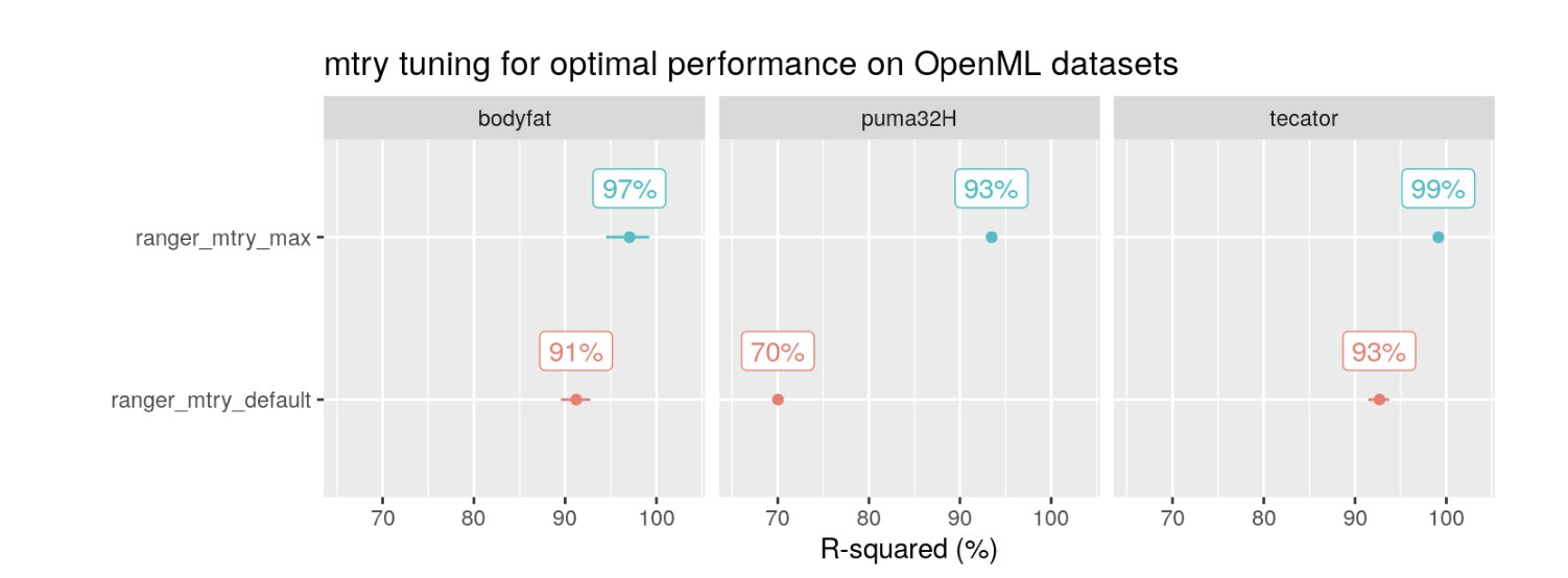
mtry: The number of potential features that can get split at each node
Most influential hyperparameter for random forests.
Increasing it improves performance in the presence of noise
Similar improvements can be had with (explicit) feature selection (e.g. recursive feature elimation)
Default:
{ranger}: \(\sqrt{p}\) , square root of the number of features
Range
{1, . . . , p}
replace: Should observations be sampled with or without replacement
Default
{ranger}: TRUE
sample.fraction: The proportion of randomly sampled observations
Default
{ranger}: 1 if replace = TRUE, 0.632 if replace = FALSE
Parameters are listed from most to least important
Seems like the strategy should be to tune structure first, then move to accuracy or overfitting parameters based on results
Missing values should be encoded as NA_integer_
Processing: it is recommended to rescale data before training so that features have similar mean and standard deviation
Hyperparameters
Structure
num_leaves: the number of decision nodes in a tree
kaggle recommendation: 2^(max_depth)
translates to a range of 8 - 4096
max_depth: The complexity of each tree
kaggle recommendation: 3 - 12
min_data_in_leaf: the minimum number of observations that fit the decision criteria in a leaf
Value depends on sample size and num_leaves
lightgbm doc recommendation: 100 - 10000 for large datasets
linear_tree (docs): fits piecewise linear gradient boosting tree
Tree splits are chosen in the usual way, but the model at each leaf is linear instead of constant
The first tree has constant leaf values
Helps to extrapolate linear trends in forecasting
Categorical features are used for splits as normal but are not used in the linear models
Increases memory use; no L1 regularization
Accuracy
n_estimators: controls the number of decision trees
learning_rate: step size parameter of the gradient descent
Kaggle recommendation: 0.01 - 0.3
Moving outside this range is usually towards zero
max_bin: controls the maximum number of bins that continuous features will bucketed into
default = 255
Overfitting
lambda_l1, lambda_l2: regularization
Default: 0
Kaggle recommendation: 0 - 100
min_gain_to_split: the reduction in training loss that results from adding a split point
Default: 0
Extra regularization in large parameter grids
Reduces training time
bagging_fraction: randomly select this percentage of data without resampling
Default: 1
* must set bagging_freq to an integer *
feature_fraction: specifies the percentage of features to sample from when training each tree
Default: 1
* Must set bagging_freq to an integer *
bagging_freq: frequency for bagging
Default: 0 (disabled)
(Integer) e.g. Setting to 2 means perform bagging at every 2nd iteration
stopping_rounds: early stopping
Issues (from docs)
Poor Accuracy
Use large max_bin (may be slower)
Use small learning_rate with large num_iterations
Use large num_leaves (may cause over-fitting)
Use bigger training data
Overfitting
Use small max_bin
Use small num_leaves
Use min_data_in_leaf and min_sum_hessian_in_leaf
Use bagging by set bagging_fraction and bagging_freq
Use feature sub-sampling by set feature_fraction
Use bigger training data
Try lambda_l1, lambda_l2 and min_gain_to_split for regularization
Try max_depth to avoid growing deep tree
Try extra_trees
Try increasing path_smooth
XGBoost
Notes
Drob starts with learning_rate = 0.01 and tune other parameters before coming back to tune learning rate
Dancho tunes learning_rate first which he says is responsible for about 80% of the model’s performance. Then, he fixes the tuned learning rate and tunes the rest of the grid of hyperparameters.
Cuts training time by 10x
Kuhn suggests setting trees to about 500 and tune stop_iter
stop_iter: early stopping; stops if no improvement has been made after this many iterations
Uber found that the most important hyperparameters were:
Details on performance, durations, etc. between sequential and simultaneous tuning methods
Links to repo, experimental paper
tldr;
They like the simultaneous tuning because had the best metric performance with the lowest variance (more stable results)
I think the sequential tuning method was comparable (and better in some cases) to the simultaneous tuning method but is probably faster and less costly.
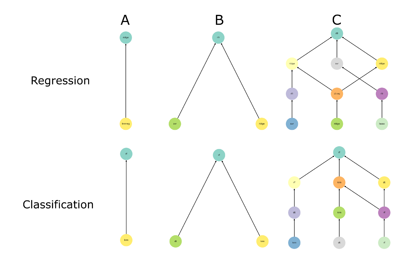
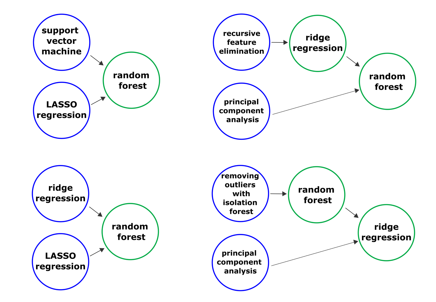
Composite Structures
W/sequential model pipelines (bottom to top)
“dtr” = decision tree regression
W/feature engineering models
On the left side are typical structures with individual predictive models being fed into an ensemble model (e.g. Random Forest)
On the right side, some kind of feature engineering process or modeling happens prior to the predictive model/ensemble model.
Sequential Tuning
Only one model is tuned at a time
The scoring, during the tuning process, happens on the ensemble model
Example
Structure
(top pipe) KNN feeds its predictions to the ridge regression which feeds it’s predictions to the lasso regression (ensemble model)
(bottom pipe) Ridge regression feeds its predictions to the random forest which feeds it’s predictions to the lasso regression (ensemble model)
Red arrows indicate how far the data/predictions have travelled through the structure. Here it’s all the way to the ensemble model
Red circle indictates which model is currently being tuned
Models without hyperparameter values are models with default values for their hyperparameters
Figure shows that the KNN and the RR (bottom pipe) models have already been tuned and the RR model (top pipe) is the model being tuned.
The red Y’ indicates that the prediction scoring, while ridge regression is being tuned, is happening at the ensemble model.
RF gets tuned next then finally the ensemble model
Simultaneous Tuning
All models, including the ensemble model, are tuned at the same time
Computationally expensive
I’d think it would be more monetarily expensive as well given that you likely have to provision more machines in any realistic scenario to get a decent training time (one for each pipe?)
Example
See Sequential tuning example for details on the structure and what items in the figure represent.
DL
Increasing or decreasing the number of training iterations
learning_rate - The gradient descent learning rate, also called \(\eta\) pr \(\alpha\)
Learning Rate Scheduling (article): The schedule reduces the learning rate as training progresses, so take smaller step sizes near and around the optimum
.png)
.png)