Feature Selection

Misc

• Why?
  • Reduces chances of overfitting
  • Multicollinearity among predictors blows up std.errors in regression
  • Lowers computer resources requirements and increase speed
• Packages
  • {Rdimtools} - Has many algorithms for feature selection
• Never use stepwise (backwards, forwards, etc.) for selecting variables according to statistical significance (e.g. p-value, or reduce the Akaike Information Criterion, or increase adjusted R-squared, or in fact any other data-driven statistics) for prediction or inferential models.
  • See Step Away From Stepwise, Stepwise selection of variables in regression is Evil
  • Some real explanatory variables that have causal effects on the dependent variable may happen to not be statistically significant, while nuisance variables may be coincidentally significant. As a result, the model may fit the data well in-sample, but do poorly out-of-sample.
  • Stepwise regression is less effective the larger the number of potential explanatory variables.
  • False positives go up and estimates are biased away from zero
  • From Harrell’s RMS
    • The R-squared or even adjusted R-squared values of the end model are biased high.
    • The F and Chi-square test statistics of the final model do not have the claimed distribution.
    • The standard errors of coefficient estimates are biased low and confidence intervals for effects and predictions are falsely narrow.
    • The p values are too small (there are severe multiple comparison problems in addition to problems 2. and 3.) and do not have the proper meaning, and it is difficult to correct for this.
    • The regression coefficients are biased high in absolute value and need shrinkage but this is rarely done.
    • Variable selection is made arbitrary by collinearity.
    • It allows us to not think about the problem.

Basic

• Harrell: Use the full model unless p > m/15 → number_of_columns > number_of_rows / 15
  • If p > m/15, then use penalyzed regression (see below, Shrinkage Methods)
• VIF - eliminate low variance predictors 
  • {collinear} - Allows you to set thresholds for correlation between predictors and VIF. The algorithm removes predictors based on those thresholds. For selecting between highly correlated variables, you can manually list the variables in order of preference or select from a few GOF functions that will be used to choose between collinear variables. Categoricals are target encoded as a preprocessing step.
• Remove Noisy Features - Compare correlation between a variable in training set and same variable in test set
• Best subset
  • {lmSubsets}: for linear regression; computes best set of predictors by fitting all subsets; chooses based on metric (AIC, BIC, etc.)
  • {leaps::regsubsets} performs best subset selection for regression models using RSS. summary(obj) gives best subset of variables for different sized subsets. nvmax arg can be used set the max size of the subsets.
  • Likelihood Ratio Test (LR Test) - For a pair of nested models, the difference in −2ln L values has a χ2 distribution, with degrees of freedom equal to the difference in number of parameters estimated in the models being compared.
    • See Diagnostics, GLM >> Deviance Metrics
• If multicollinearity is a problem
  • Reduction methods - PCA
  • Shrinkage methods - lasso, ridge, elastic net, Least Angle Regression (LAR)
  • ML
    • Fuzzy Forests (See below)
    • Oblique Forests
      • Article on {bonsai} implementation of {aorsf} through {tidymodels}
      • Regression, Survival >> ML >> Random Survival Forests >> {aorsf}

Complex

• Projection Predictive
  • {projpred} (Vehtari)
  • It is variable selection for various regression models, and also allows for valid post-selection inference
  • Papers and other articles in bkmks >> Features >> Selection >> projpred
  • Currently requires {rstanarm} or {brms} models
  • Families: gaussian, binomial, poisson. Also categorical and ordinal
  • Terms: linear main effects, interactions, multilevel, other additive terms
  • Components
    • Search: determines the solution path, i.e., the best submodel for each submodel size (number of predictor terms).
    • Evaluation: determines the predictive performance of the submodels along the solution path
  • After model selection, a matrix of projected posterior draws is produced using the reference model and the selected number of features. Then, typical posterior stats for variable effects can be calculated, visualized via {posterior}, {bayesplot}, etc.
    • Projected Posterior Distribution - The distribution arising from the deterministic projection of the reference model’s posterior distribution onto the parameter space of the final submodel
  • Also see Horseshoe model
    • Regularized Horseshoe prior
    • Gelman - link
    • Paper
• Multi-Layer Group-Lasso
  • This approach combines variable aggregation and selection in order to improve interpretability and performance
  • {MLGL}
  • Goal is to remove redundant variables from a high dim dataset.
  • Steps
    1. A hierarchical clustering procedure provides at each level a partition of the variables into groups.
    2. The set of groups of variables from the different levels of the hierarchy is given as input to group-Lasso, with weights adapted to the structure of the hierarchy.
       • At this step, group-Lasso outputs sets of candidate groups of variables for each value of the regularization parameter
• Ensemble Ranking
  
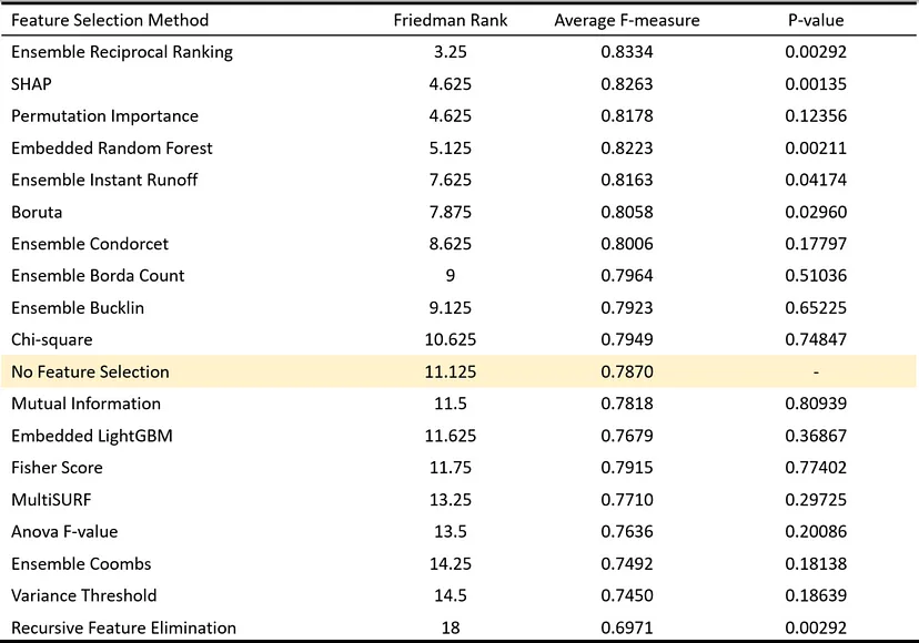
  • Apply multiple feature selection methods then create an ensemble ranking
  • Paper, Article
    • Compared 12 individual feature selection methods and the 6 ensemble methods described above in 8 datasets for a classification task
  • Best performance is Ensemble Reciprocal Ranking
    \[ r(f) = \frac{1}{\sum_j \frac{1}{r_j(f)}} \]
    • \(r(f)\) is the final rank of feature \(f\)
      • \(j\) is the the index for the feature selection methods
    • Equivalent to the harmonic mean rank
    • aka Inverse Rank Position
    • Lower is better (I think)
  • Best performance by single method is SHAP
• Boruta
  • Built around random forest algorithm Can identify variables involved in non-linear interactions. Slow if dealing with thousands of variables
  • {Boruta}
• Multivariable Fractional Polynomials
  • Fits polynomial transformations of features with exponents in a range of numbers including fractions
  • Includes a pretty intensive statistical model testing procedure
  • {mfp}, Explainer
• Component-wise Boosting
  • {bounceR}
  • Article, Video
  • Uses component-wise boosting from {mboost} to score features and selects features with aggregate scores beyond some kind of threshold.
  • It’s not well-explained at all and there is only documentation on how to use it. I haven’t watched the video, so that could possibly explain the method better.
  • See Algorithms, ML >> Boosting >> XGBoost for details on mboost’s algorithm
  • Also has bivariate comparison methods: correlation, zero-variance, and information criteria
• Reversible Jump MCMC (RJMCMC)
  • Variable selection in NIMBLE using reversible jump MCMC
    • Brief explanation and example
  • A general framework for MCMC simulation in which the dimension of the parameter space (i.e., the number of parameters) can vary between iterations of the Markov chain.
• Fuzzy Forests
  • Extends Random Forest Feature Selection for Correlated, High-Dimensional Data
  • {fuzzyforest}
  • Uses recursive feature elimination random forests to select features from separate blocks of correlated features where the correlation within each block of features is high and the correlation between blocks of features is low.
  • Then, one final random forest is fit using the surviving features.
• Gain Penalyzed Forests

  • Uses gain penalization to regularize the random forest algorithm

  • Think this also works for numeric target variables

  • Notes from

    • Feature Selection via Gain Penalization in Random Forests
      • Includes coded example
    • Paper

  • When determining the next child node to be added to a decision tree, the gain (or the error reduction) of each feature is multiplied by a penalization parameter
    \[ \mbox{Gain}_R(\boldsymbol{X}_i, t) = \left\{ \begin{array}{lcl} \lambda \Delta(i, t) & i \notin \mathbb{U} \\ \Delta(i,t) & i\in \mathbb{U} \end{array}\right. \]

    • \(U\) is the set of indices of the features previously used in the tree
    • \(X_i\) is the candidate feature
    • \(t\) is the candidate splitting point
    • \(\lambda\) is the penalty for each variable, \(\lambda \in (0,1]\) (See below)
    • So at each split point, variables that have NOT been chosen at prior split points receive a penalty

  • Penalty for each variable (the λ shown in the Gain equation above)

    \[ \lambda = (1-\gamma)\cdot\lambda_0 + \gamma \cdot g(x_i) \]

    • \(\lambda_i \in [0,1)\)
    • \(\lambda_0 \in [0,1)\) is interpreted as the baseline regularization
    • \(\gamma \in [0,1)\) is the mixture parameter
    • \(g(x_i)\) is a function of the i^th feature
      • Should represent relevant information about the feature, based on some characteristic of interest (correlation to the target, for example)
      • Introduces “prior knowledge” regarding the importance of each feature into the model
      • The data will tell us how strong our assumptions about the penalization are, since even if we try to penalize a truly important feature, its gain will be high enough to overcome the penalization and the feature will get selected by the algorithm
      • Examples
        • The Mutual Information between each feature and the target variable \(y\)
          • Normalized to be between 0 and 1
        • The variable importance values obtained from a previously run standard Random Forest, which is what I call a Boosted g(xi)
          • Normalized to be between 0 and 1
        • Other options, see the paper

  • Steps

    1. We run a bunch of penalized random forests models with different hyperparameters and record their accuracies and final set of features
       • \(\gamma\), \(\lambda_0\) and mtry are hyperparameters that should be tuned
    2. For each training dataset, select the top-n (e.g. n = 3) fitted models in terms of the accuracies, and run a “new” random forest for each of the feature sets used by them. This is done using all of the training sets so we can evaluate how these features perform in slightly different scenarios
    3. Finally, get the top-m set of models (here m = 30) from these new ones, check which features were the most used between them and run a final random forest model with this feature set.
       • e.g. Select only the 15 most used features from the top 30 models, but both numbers can be changed depending on the situation
• Distance Correlation Forward Selection
  • Also see Regression, Regularized >> Misc >> Variable Selection
  • “The distance correlation algorithm for variable selection (DC.VS) of Febrero-Bande et al. (2019). This makes use of the correlation distance (Székely et al., 2007; Szekely & Rizzo, 2017) to implement an iterative procedure (forward) deciding in each step which covariate enters the regression model.”
  • Starting from the null model, the distance correlation function, dcor.xy,  in {fda.usc} is used to choose the next covariate
    • Guessing you want large distances between an already chosen variable and the next variable
    • Maybe for the first explanatory variable you want a short distance between the it and the outcome variable
    • Dunno what the stopping criteria is
  • Algorithm discussed in this paper, Variable selection in Functional Additive Regression Models

Multidimensional Feature Selection (MDFS)

• Misc

  • {mdfs} and {{mdfs}} - Vignette, Paper

    • There’s a mention of CUDA, so this could be GPU-capable

• Description

  • Compares tuples of variables using entropy/information gain (see below for details on the algorithm)

  • A filter method which means it identifies informative variables before modelling is performed.

    • In general, filter methods are usually simplistic and therefore fast, but simplicity can sometimes lead to errors

  • As of 2019-10-13, implementation only for use with binary outcomes

    • For multi-categorical outcomes, vignette suggests either performing the analyses with all pairs of outcome categories, then any variable deemed relevant for one analysis is considered relevant. Instead of doing all-pairs, you can dichotomize variable into pairs of category-other which would be less expensive
    • Continuous outcomes have to be discretized

  • The algorithm explores all k-tuples of variables for k-dimensional analysis

    \[ x \cup \{x_{m_1}, x_{m_2}, \ldots, x_{m_{k-1}}\} \]

    • \(x_i\) is one of the explanatory variables
    • The max k is 5
      • If it’s GPU-capable, this may not be the case anymore
      • For larger values than 5, it becomes computationally expensive and detecting significant differences in conditional entropy becomes less likely.
      • For example, 2-dimensional analysis would explore the set of all possible pairs (2-tuples) of variables.
        • For each variable, \(x_i\), check whether adding it to the set with another variable, \(x_j\), adds information to the system.
        • If there exists such a \(x_j\), then we declare \(x_i\) as 2-weakly relevant.

• Steps

  1. Discretize all variables
     • Choose the number of classes, \(c\)
       • All variables are coerced into having the same number of classes (even binary? So if you have one binary, then all variables are coerced into binaries?)
       • Unless there’s domain knowledge, multiple \(c\) values should be tried.
     • Randomly sample (\(c-1\)) integers from a uniform distribution on the interval, (\(2, N\)) where \(N\) is the number of observations.
       • The integers will be indexes where the variable is split into c classes
       • At first glance it looks like the interval starts at 2 so that each class has minimum of 2 or 3 values (depending if the split happens before or after the integer), but unless there’s some kind of check, two consecutive integers, like 19,20, could still be sampled and then you have a problem. With a large data set, it seems unlikely to happen, but it’d still be possible. So I don’t know why it starts at 2. The vignette isn’t clear about this IMO.
     • Sort the variable
       • I guess smallest value to largest? Probably doesn’t matter as long as it’s consistent for all variables)
     • Split the sorted variable at the indexes given by the randomly sampled integers
     • Repeat for each variable
       • The outcome variable might have to be done manually by the user prior to starting analysis/
  2. Compute conditional entropy for Y given the k-dimension variable set that includes a specific variable and the conditional entropy for the (\(k-1\)) set that excludes that specific variable.

     • Conditional Entropy for \(Y | X_1, \ldots, X_k\) is

       \[ H(Y|X_1, \ldots, X_k) = \sum_{d=0} \sum_{i_1 = 1}^c \ldots \sum_{i_k = 1}^c P(y_d | x_{i_1}, \ldots, x_{i_k}) \; \log P(y_d |x_{i_1}, \ldots, x_{i_k}) \]

       • \(d\) is for the outcome variable category which much be binary
       • \(i_1\) is the ith category of the 1^st variable
       • \(i_k\) is the ith category of the k^th variable
       • This sequence of summations amounts to taking every permutation of outcome category and every category of every explanatory variable and summing them together.
       • See the Algorithms, ML >> Trees >> Decision Trees for further discussion
       • The conditional entropy for the (\(k-1\)) set of explanatory variable is calculated similarily

     • If \(k\) is less than total number of variables, then this process could include many permutations

  3. Compute the mutual information gain between these two entropies. Then out of all the mutual information values from all the different permutations of the \(k\)-tuple, choose the maximum value

     • Mutual information is the difference between two conditional entropies. Very similar to the information gain used in trees

       \[ IG_{\max}^k = N \; \max \{H(Y|X_1, \ldots, X_k) - H(Y|X_1, \ldots, X_{k-1})\} \]

       • \(m\) is m^th permutation of the \(k\)-tuple
       • \(N\) is the number of observations. The reason for it being there is that multiplying the \(IG_{\max}\) by \(N\) makes it a distribution parameter that can be hypothesis tested.
  4. Hypothesis test this difference (\(IG_{\max}\)) to see if it’s significant
     • If the difference is significant, then that variable is k-weakly relevant
     • Test statistic for a specific \(\alpha\)-level is from an empirically calculated distribution
     • Adjust p-values to control FWER or FDR
  5. If performing a more complicated model selection process, take the top n variables whose \(IG_{\max}\) was significant and repeat steps
     • Guessing this is backwards elimination
     • This is a method that’s built for dealing with thousands of variables, so this taking top-n-then-repeat seems to be a way of controlling the amount of time needed to complete the analysis.