Lakes
Misc
- Data is stored in structured format or in its raw native format without any transformation at any scale.
- Handling both types allows all data to be centralized which means it can be better organized and more easily accessed.
- Optimal for fit for bulk data types such as server logs, clickstreams, social media, or sensor data.
- Ideal use cases
- Backup for logs
- Raw sensor data for your IoT application,
- Text files from user interviews
- Images
- Trained machine learning models (with the database simply storing the path to the object)
- Tools
- Rclone - A command-line program to manage files on cloud storage. It is a feature-rich alternative to cloud vendors’ web storage interfaces. Over 70 cloud storage products support rclone including S3 object stores
- {pins}, {pins}
- Posit’s Pins Docs
- Articles
- Automating data updates with R: Tracking changes in a GitHub-hosted dataset
- Pulls sha from dataset repo and compares to the old one to determine if data needs update. Logs the sha and any error messages with {logger}. If there’s new data, uses {pins} to download dataset and version it.
- There’s not much to this script, but I think {git2r} might’ve been nicer that using {httr} and {jsonlite} to manually pull from the github API
- Automating data updates with R: Tracking changes in a GitHub-hosted dataset
- Convenient storage method
- Can be used for caching
- Can be automatically versioned, making it straightforward to track changes, re-run analyses on historical data, and undo mistakes
- Needs to be manually refreshed
- i.e. Update data model, etc. and run script that rights it to the board.
- Use when:
- Object is less than a 1 Gb
- Use {butcher} for large model objects
- Some model objects store training data
- Use {butcher} for large model objects
- Object is less than a 1 Gb
- Benefits
- Just need the pins board name and name of pinned object
- Think the set-up is supposed to be easy
- Easy to share; don’t need to understand databases
- Just need the pins board name and name of pinned object
- Boards
Folders to share on a networked drive or with services like DropBox
Posit Connect, Amazon S3, Google Cloud Storage, Azure storage, Databricks and Microsoft 365 (OneDrive and SharePoint)
Example: Pull data, clean and write to board
board <-
  pins::board_connect(
    auth = "manual",
    server = Sys.getenv("CONNECT_SERVER"),
    key = Sys.getenv("CONNECT_API_KEY")
  )

# code to pull and clean data

pins::pin_write(board = board,
                x = clean_data,
                name = "isabella.velasquez/shiny-calendar-pin")
- obstore: The simplest, highest-throughput Python interface to S3, GCS & Azure Storage, powered by Rust.
- Features
- Easy to install with no Python dependencies.
- Sync and async API.
- Streaming downloads with configurable chunking.
- Automatically supports multipart uploads under the hood for large file objects.
- The underlying Rust library is production quality and used in large scale production systems, such as the Rust package registry crates.io.
- Simple API with static type checking.
- Helpers for constructing from environment variables and
boto3.Sessionobjects
- Supported object storage providers include:
- Amazon S3 and S3-compliant APIs like Cloudflare R2
- Google Cloud Storage
- Azure Blob Gen1 and Gen2 accounts (including ADLS Gen2)
- Local filesystem
- In-memory storage
- Features
- Lower storage costs due to their more open-source nature and undefined structure
- On-Prem set-ups have to manage hardward and environments
- If you wanted to separate stuff like test data from production data, you also probably had to set up new hardware.
- If you had data in one physical environment that had to be used for analytical purposes in another physical environment, you probably had to copy that data over to the new replica environment.
- Have to keep a tie to the source environment to ensure that the stuff in the replica environment is still up-to-date, and your operational source data most likely isn’t in one single environment. It’s likely that you have tens — if not hundreds — of those operational sources where you gather data.
- Where on-prem set-ups focus on isolating data with physical infrastructure, cloud computing shifts to focus on isolating data using security policies.
- Object Storage Systems
- Cloud data lakes provide organizations with additional opportunities to simplify data management by being accessible everywhere to all applications as needed
- Organized as collections of files within directory structures, often with multiple files in one directory representing a single table.
- Pros: highly accessible and flexible
- Metadata Catalogs are used to answer these questions:
- What is the schema of a dataset, including columns and data types
- Which files comprise the dataset and how are they organized (e.g., partitions)
- How different applications coordinate changes to the dataset, including both changes to the definition of the dataset and changes to data
- Hive Metastore (HMS) and AWS Glue Data Catalog are two popular catalog options
- Contain the schema, table structure and data location for datasets within data lake storage
- Issues:
- Does not coordinate data changes or schema evolution between applications in a transactionally consistent manner.
- Creates the necessity for data staging areas and this extra layer makes project pipelines brittle
- Does not coordinate data changes or schema evolution between applications in a transactionally consistent manner.
Terms
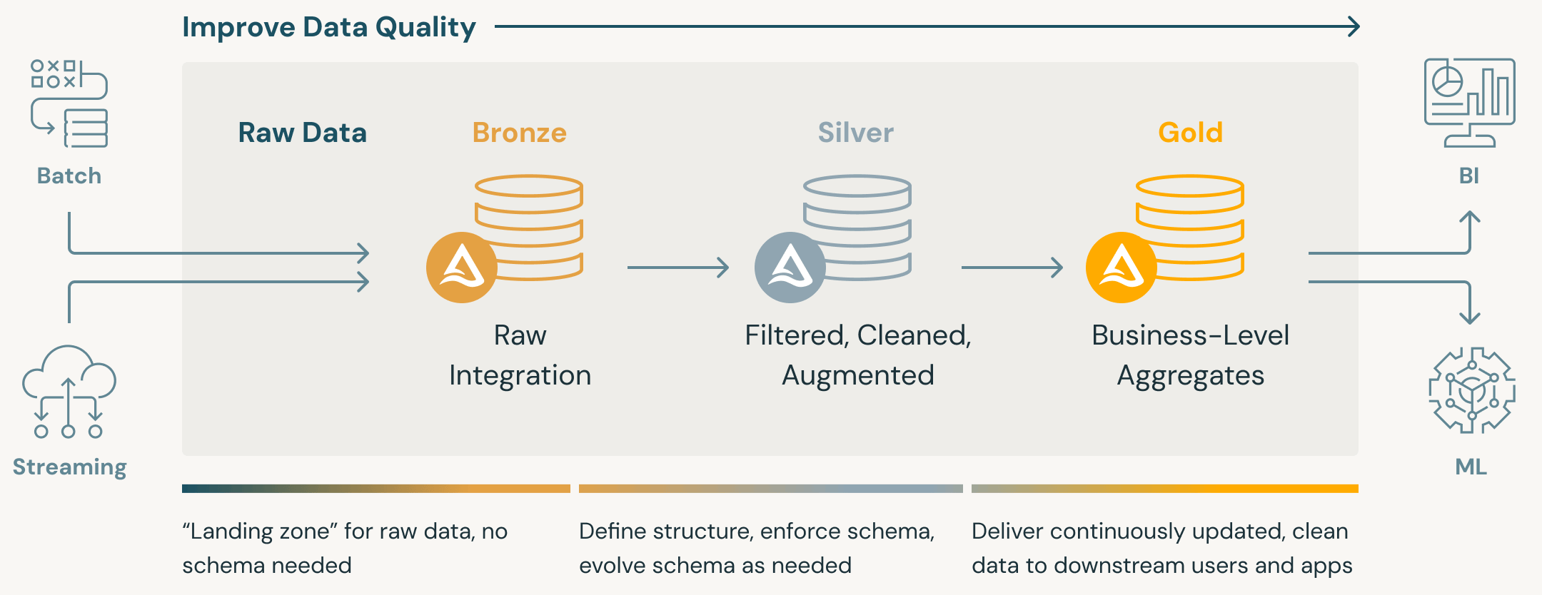
Medallion Architecture - A data design pattern used to logically organize data in a lakehouse, with the goal of incrementally and progressively improving the structure and quality of data as it flows through each layer of the architecture (from Bronze ⇒ Silver ⇒ Gold layer tables). (source)
- Also see
- Ducklake >> R >> Example 2
- Medallion architectures are sometimes also referred to as “multi-hop” architectures.
- Compatible with the concept of a data mesh. Bronze and silver tables can be joined together in a “one-to-many” fashion, meaning that the data in a single upstream table could be used to generate multiple downstream tables
- Bronze: Data from external source systems.
- The table structures in this layer correspond to the source system table structures “as-is,” along with any additional metadata columns that capture the load date/time, process ID, etc.
- The focus in this layer is quick Change Data Capture and the ability to provide an historical archive of source (cold storage), data lineage, auditability, reprocessing if needed without rereading the data from the source system.
- Silver: Data from the Bronze layer is matched, merged, conformed and cleansed (“just-enough”) so that the Silver layer can provide an “Enterprise view” of all its key business entities, concepts and transactions. (e.g. master customers, stores, non-duplicated transactions and cross-reference tables).
- Enables self-service analytics for ad-hoc reporting, advanced analytics and ML.
- Only minimal or “just-enough” transformations and data cleansing rules are applied while loading the Silver layer
- Has more 3rd-Normal Form like data models.
- Data Vault-like where write-performant data models can be used in this layer
- Gold: Consumption-ready “project-specific” databases
- For reporting and uses more de-normalized and read-optimized data models with fewer joins. Data quality rules are applied here.
- Final presentation layer of projects such as Customer Analytics, Product Quality Analytics, Inventory Analytics, Customer Segmentation, Product Recommendations, Marking/Sales Analytics etc.
- Kimball style star schema-based data models or Inmon style Data marts are often used
- Also see
Brands
- Amazon S3
- Add a hash to your bucket names and explicitly specify your bucket region!!
- Try to stay <1000 entries per level of hierarchy when designing the partitioning format. Otherwise there is paging and things get expensive.
- AWS Athena ($5/TB scanned)
- AWS Athena is serverless and intended for ad-hoc SQL queries against data on AWS S3
- Apache Hudi - A transactional data lake platform that brings database and data warehouse capabilities to the data lake. Hudi reimagines slow old-school batch data processing with a powerful new incremental processing framework for low latency minute-level analytics.
- Azure
- Data Lake Storage (ADLS)
- Packages
- {quak} - Provides convenience utilities for using ‘DuckDB’ directly over datasets stored in ‘Azure Data Lake Storage Gen2’
- Big data analytics workloads (Hadoop, Spark, etc.)
- ADLS Gen2 uses a hierarchical namespace which mimics a directory structure (e.g., folders/files). This enables high-performance analytics scenarios.
- Supports HDFS-like interface (e.g. Hadoop)
- Optimized for Azure Synapse, Databricks, HDInsight
- ADLS Gen2 is built on top of Blob Storage, so you pay the same base storage costs plus some for additional capabilities.
- Use Cases
- Building a data lake for analytics workloads
- Integrating with Spark, Synapse, Databricks
- Packages
- Blob Storage - Massively scalable and secure object storage for cloud-native workloads, archives, data lakes, HPC, and machine learning
- Azure’s S3
- General-purpose object storage (images, docs, backups, etc.)
- Use Cases:
- Web/mobile app data, backups, media files
- Archiving and static content delivery
- Data Lake Storage (ADLS)
- Garage - An open-source distributed object storage service tailored for self-hosting
hrbrmstr blessed, “minimal, resilient object store designed to live across your homelab nodes without demanding Kubernetes clusters or a Ph.D. in consensus algorithms. … Garage makes sense when you want to spread data across a few sites, stay independent of big-cloud object stores, and avoid the maintenance gravity of MinIO clusters.”
Example: Querying w/{duckdb, dplyr} (source)
Code
library(duckdb)
library(dplyr)

con <- dbConnect(duckdb::duckdb())

dbExecute(con, sprintf(r"(
INSTALL httpfs;
LOAD httpfs;
SET s3_endpoint='%s';
SET s3_access_key_id='%s';
SET s3_secret_access_key='%s';
SET s3_use_ssl=false;
SET s3_url_style='path';
SET s3_region='garage';
)",
  Sys.getenv("garage_s3_endpoint"),
  Sys.getenv("garage_s3_access_key_id"),
  Sys.getenv("garage_s3_secret_access_key")
))

tbl(con, sql(r"(
FROM (
  FROM (
    FROM read_parquet('s3://tspq/dt=*/*.parquet', hive_partitioning=true)
    SELECT
      substring(dt, 1, 10)::DATE AS day,
      ip,
      UNNEST(internet_scanner_intelligence)
    WHERE dt >= '2025-09-01-00'
  )
  SELECT
  * EXCLUDE(metadata),
  UNNEST(metadata)
)
SELECT
  * EXCLUDE(raw_data),
  UNNEST(raw_data)
)"))

## # Source:   SQL [?? x 46]
## # Database: DuckDB v1.2.2 [root@Darwin 25.1.0:R 4.5.0/:memory:]
##    day        ip          first_seen last_seen found tags  actor
##    <date>     <chr>       <chr>      <chr>     <lgl> <lis> <chr>
##  1 2025-09-01 1.0.165.243 2020-03-11 2025-09-… TRUE  <chr> unkn…
##  2 2025-09-01 1.0.211.172 2020-11-10 2025-09-… TRUE  <chr> unkn…
##  3 2025-09-01 1.0.226.5   2025-08-31 2025-09-… TRUE  <chr> unkn…
##  4 2025-09-01 1.0.235.31  2020-12-25 2025-09-… TRUE  <chr> unkn…
##  5 2025-09-01 1.0.235.44  2025-08-31 2025-09-… TRUE  <chr> unkn…
##  6 2025-09-01 1.0.248.134 2019-11-25 2025-09-… TRUE  <chr> unkn…
##  7 2025-09-01 1.0.249.246 2021-05-25 2025-09-… TRUE  <chr> unkn…
##  8 2025-09-01 1.0.251.21  2025-08-31 2025-09-… TRUE  <chr> unkn…
##  9 2025-09-01 1.0.251.93  2024-08-09 2025-09-… TRUE  <chr> unkn…
## 10 2025-09-01 1.0.253.141 2024-05-27 2025-09-… TRUE  <chr> unkn…
## # ℹ more rows
## # ℹ 39 more variables: spoofable <lgl>, classification <chr>,
## #   cves <list>, bot <lgl>, vpn <lgl>, vpn_service <chr>,
## #   tor <lgl>, last_seen_timestamp <chr>, asn <chr>,
## #   source_country <chr>, source_country_code <chr>,
## #   source_city <chr>, domain <chr>, rdns_parent <chr>,
## #   rdns_validated <lgl>, organization <chr>, category <chr>, …
## # ℹ Use `print(n = ...)` to see more rows
- Google Cloud Storage
- 5 GB of US regional storage free per month, not charged against your credits.
- Hadoop
- Traditional format for data lakes
- Linode/Akaime Cloud S3
- MinIO (Put into maintenance mode)
- Open-Source alternative to AWS S3 storage.
- Given that S3 often stores customer PII (either inadvertently via screenshots or actual structured JSON files), Minio is a great alternative to companies mindful of who has access to user data.
- Of course, AWS claims that AWS personnel doesn’t have direct access to customer data, but by being closed-source, that statement is just a function of trust.
- RustFS - An open-source, S3-compatible high-performance object storage system supporting migration and coexistence with other S3-compatible platforms such as MinIO and Ceph
- SeaweedFS - A fast distributed storage system for blobs, objects, files, and data lake, for billions of files
- Blob store has O(1) disk seek, cloud tiering. Filer supports Cloud Drive, xDC replication, Kubernetes, POSIX FUSE mount, S3 API, S3 Gateway, Hadoop, WebDAV, encryption, Erasure Coding.
- Enterprise version is at seaweedfs.com.
- Wasabi Object Storage
- $7/month per terabyte
Lakehouses
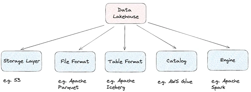
- The key idea behind a Lakehouse is to be able to take the best of a Data Lake and a Data Warehouse.
- Data Lakes can in fact provide a lot of flexibility (e.g. handle structured and unstructured data) and low storage cost.
- Data Warehouses can provide really good query performance and ACID guarantees.
- Pipeline
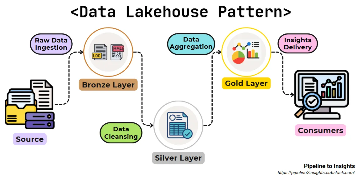
- Purpose: Blends the structured querying capabilities of data warehouses with the flexibility and scalability of data lakes.
- Method: Organizes data into three layers (Medallion Architecture):
- Bronze Layer: Stores raw data in its original form.
- Silver Layer: Cleansed and validated data ready for further analysis.
- Gold Layer: Analytics-ready data refined for specific business use cases.
- Benefits:
- Provides unified analytics across structured and semi-structured data.
- Reduces duplication by combining data lake and warehouse capabilities.
- Limitations: Requires careful management of data across the three layers to avoid inconsistencies and inefficiencies.
Apache Iceberg
- Open source table format that addresses the performance and usability challenges of using Apache Hive tables in large and demanding data lake environments.
- Other currently popular open table formats are Hudi and Delta Lake.
- Packages
- Resources
- Comparison between Delta Lake and Iceberg tablle local set-up
- A bit outdated (dec 2024) when I read it as more python packages have now started supporting iceberg, but the set-up code for Iceberg might still be useful.
- Comparison between Delta Lake and Iceberg tablle local set-up
- Interfaces
- Features
- Transactional consistency between multiple applications where files can be added, removed or modified atomically, with full read isolation and multiple concurrent writes
- Full schema evolution to track changes to a table over time
- Time travel to query historical data and verify changes between updates
- Partition layout and evolution enabling updates to partition schemes as queries and data volumes change without relying on hidden partitions or physical directories
- Rollback to prior versions to quickly correct issues and return tables to a known good state
- Advanced planning and filtering capabilities for high performance on large data volumes
- The full history is maintained within the Iceberg table format and without storage system dependencies
- Issues (source)
- Uses O(n) operations to add new metadata to an existing table - where it should have used O(1) or O(log(n))
- Cannot handle cross table commits
- Relies on file formats that are bloated and ineffective
- Tries to be a “file only” format, but still needs a database to operate
- Does not handle fragmentation and metadata bloat and remains silent about the real complexities of that problem
- Does not handle row level security or security at all for that matter
- Fundamentally does not scale - because it uses a bad, optimistic concurrency model
- Is entirely unfit for trickle feeding of data - a hallmark feature of large Data Lakes
- Moves an extraordinary amount of complexity (and trust) to the client talking to it
- Makes proper caching and query planning (the hallmarks of good analytics) very difficult, if not impossible
- Components
- Iceberg Catalog - Used to map table names to locations and must be able to support atomic operations to update referenced pointers if needed.
- For keeping track of external files and updating/changing data while keeping track of file locations and names.
- Metadata Layer (with metadata files, manifest lists, and manifest files) - Stores instead all the enriching information about the constituent files for every different snapshot/transaction
- e.g. table schema, configurations for the partitioning, etc.
- Data Layer - Associated with the raw data files
- Iceberg Catalog - Used to map table names to locations and must be able to support atomic operations to update referenced pointers if needed.
- Supports common industry-standard file formats, including Parquet, ORC and Avro
- Supported by major data lake engines including Dremio, Spark, Hive and Presto
- Queries on tables that do not use or save file-level metadata (e.g., Hive) typically involve costly list and scan operations
- Any application that can deal with parquet files can use Iceberg tables and its API in order to query more efficiently
- Comparison
.png)
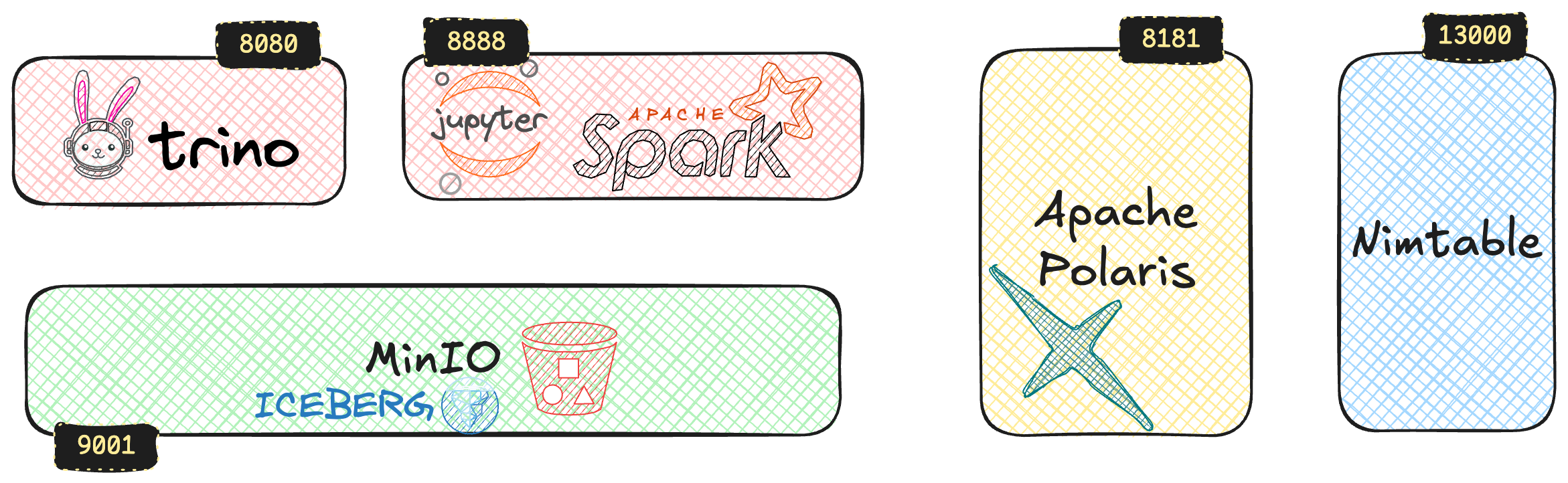
- Stacks
Delta Lake
- Databricks closed source table format. Very similar to Iceberg, but slightly more popular and supported (i.e. read/write) by more packages. Its Unity catalogue can be easier to set up as well.
- Docs
- Packages
- Deletion Vectors - DELETE, UPDATE, and MERGE operations use deletion vectors to mark existing rows as removed or changed without rewriting the Parquet file. Subsequent reads on the table resolve the current table state by applying the deletions indicated by deletion vectors to the most recent table version.
- By default, when a single row in a data file is deleted, the entire Parquet file containing the record must be rewritten.
DuckLake
- Notes from
- Resources
- Docs, Intro (with examples)
- Catalog Database Options and Usage
- If you would like to perform local data warehousing with a single client, use DuckDB as the catalog database.
- If you would like to perform local data warehousing using multiple local clients, use SQLite as the catalog database.
- If you would like to operate a multi-user lakehouse with potentially remote clients, choose a transactional client-server database system as the catalog database: MySQL or PostgreSQL.
- Open source “catalog” format which instead of using a catalog architecture (hierarchical filing system like in Iceberg) for metadata, DuckLake uses a database to much more efficiently and effectively manage the metadata needed to support changes.
- They’re using “catalog” because it replaces the whole lakehouse stack.
- Also what Google BigQuery (with Spanner) and Snowflake (with FoundationDB) have chosen (metadata in SQL database), just without the open formats at the bottom
- Hierarchical file based metadata (Iceberg, Deltalake) runs into performance bottleneck for high frequency transactions. So it’s is now being augmented with cataloguing services such as ‘Snowflake’s Polaris over Iceberg’ or ‘Databricks Unity Catalogue over Delta’ — which adds further abstraction and complexity.
- The SQL database that hosts the catalog server can be any halfway competent SQL database that supports ACID and primary key constraints. (e.g. PostgreSQL, SQLite, MySQL and MotherDuck)
- Metadata is roughly 5 orders of magnitude smaller than your actual data: a petabyte of Parquet data requires only ~10 GB of metadata. Even at massive scale, this metadata easily fits within the capabilities of modern RDBMS systems that routinely handle terabyte-scale databases.
- Supports integration with any storage system like local disk, local NAS, S3, Azure Blob Store, GCS, etc. The storage prefix for data files (e.g.,
s3://mybucket/mylake/) is specified when the metadata tables are created. - Components (i.e. only infrastructure requirements are parquet file storage, metadata file storage)
- DuckLake Interface - Standard SQL for all operations.
- Commodity RDBMS - An ACID-compliant database, for storing metadata (PostgreSQL, SQLServer, Oracle, MySQL, SQLite, DuckDB itself).
- Parquet files - The open standard for storage of tabular data for analytics workloads for storing raw data.
- Commodity file storage - Any common platform that can act as an object store (Amazon S3, Azure Blob, Google Cloud Storage, local filesystem, etc.).
- Currently supports only NOT NULL constraints.
- PRIMARY KEY, FOREIGN KEY, UNIQUE, and CHECK constraints are not yet implemented, though this may change as the format matures.
- Frozen Ducklakes
- Notes from
- Frozen DuckLakes for Multi-User, Serverless Data Access
- Article shows an example of creating a read-only DuckDB database file and how to create new revisions of a Frozen DuckLake.
- Frozen DuckLakes for Multi-User, Serverless Data Access
- A read-only and has no moving parts other than a cloud storage system
- Advantages
- They have almost zero cost overhead on top of the storage of the Parquet data files.
- A Frozen DuckLake can be used for public-facing data (e.g., public buckets), since there are no extra services required over cloud or HTTP file access.
- They make the data immediately accessible in a SQL database with no special provisions required.
- They allow data files to live in different cloud environments, while being referenced from the same Frozen DuckLake.
- Versioning
- Data can still be updated by creating a new Frozen DuckLake.
- Older versions can be accessed by retaining revisions of the DuckDB database file — or by simply using time travel.
- Notes from
R
- Packages
- {ducklake} - Provides ACID transactions, automatic versioning, time travel queries, and complete audit trails
- Preserves relational structure between related datasets
- Automatically versions every data change with timestamps and metadata
- Enables time travel to recreate analyses exactly as they were run
- Provides complete audit trails with author attribution and commit messages
- Supports layered architecture (bronze/silver/gold) for data lineage from raw to analysis-ready
- Allows multiple team members to collaborate safely with shared data
- {ducklake} - Provides ACID transactions, automatic versioning, time travel queries, and complete audit trails
- Requires {duckdb} > version 1.3.1
- Example 1: Basic Workflow
Local Set-Up
1db_file <- file.path(tempdir(), "metadata.ducklake") 2work_dir <- file.path(tempdir(), "lake_data_files") con <- dbConnect(duckdb()) db_path <- glue_sql('{paste0("ducklake:", db_file)}', .con = con) setup_dlake_cmd <- glue::glue_sql(" INSTALL ducklake; 3 ATTACH 'ducklake:{db_file}' AS my_ducklake (DATA_PATH {work_dir}); 4 USE my_ducklake; ", .con = con) DBI::dbExecute(con, setup_dlake_cmd)- 1
- db_file is the location of the metadata database
- 2
- work_dir is the location of the data you’re working with that are stored in parquet files. db_file and work_dir could also be URLs to a cloud location on AWS S3 or within a Google Cloud bucket instead, etc.
- 3
- my_ducklake is the name of the lakehouse
- 4
-
USEsets my_ducklake as the default lakehouse
Create a Table
dbWriteTable( conn = con, name = "stats", value = dplyr::filter(stats, contrast %in% c("two_months", "four_months")) ) dbWriteTable(con, "exprs", exprs)- stats and exprs are two datasets in memory
- You can also read parquet files into duckdb
arrow::read_parquet and arrow::to_duckdb(See Databases, DuckDB >> Arrow >> Example: (using SQL Query; method 2)- DuckDB SQL:
FROMread_parquet('/Users/ercbk/Documents/R/Data/foursquare-spaces/*.parquet')(See Databases, DuckDB >> SQL >> Example 1 and dbplyr >> Example 1) duckplyr::read_parquet_duckdb(See Databases, DuckDB >> duckplyr >> Operations)
Do Work
Example: Basic
query_sym <- " SELECT contrast, COUNT(symbol) FROM my_ducklake.stats GROUP BY contrast; " df_fsq <- DBI::dbGetQuery(conn, query_sym) lazy_df <- tbl(con, "stats") |> dplyr::filter(symbol == "Cd34") lazy_df #> # Source: SQL [?? x 9] #> # Database: DuckDB v1.3.1 [root@Darwin 24.5.0:R 4.5.0/:memory:] #> study contrast symbol gene_id logFC CI.L CI.R P.Value adj.P.Val #> <chr> <chr> <chr> <chr> <dbl> <dbl> <dbl> <dbl> <dbl> #> 1 Wang_2018 two_months Cd34 ENSMUSG0000… 1.10 0.935 1.26 2.21e-14 2.23e-10 #> 2 Wang_2018 four_months Cd34 ENSMUSG0000… 1.99 1.81 2.18 6.75e-20 7.51e-17- Show two ways of querying data: DBI and dbplyr
View Data Files
query_files <- "
FROM ducklake_table_info('my_ducklake')
"
DBI::dbGetQuery(query_files)

fs::dir_info(file.path(work_dir, "main", "stats")) |>
  dplyr::mutate(filename = basename(path)) |>
  dplyr::select(filename, size)
#> # A tibble: 1 × 2
#>   filename                                                     size
#>   <chr>                                                 <fs::bytes>
#> 1 ducklake-019804b9-2259-7bf9-b53c-2ab7be53e198.parquet       1.42M
Add data to a table
dbAppendTable( conn = con, name = "stats", value = dplyr::filter(stats, contrast %in% c("six_months", "eight_months")) ) fs::dir_info(file.path(work_dir, "main", "stats")) |> dplyr::mutate(filename = basename(path)) |> dplyr::select(filename, size) #> # A tibble: 2 × 2 #> filename size #> <chr> <fs::bytes> #> 1 ducklake-019804b9-2259-7bf9-b53c-2ab7be53e198.parquet 1.42M #> 2 ducklake-019804b9-236f-71fa-ad7a-81f6e9a6f01d.parquet 1.44M- After appending the data to the stats table, we can see that an additional parquet file was created.
Detach and Disconnect
dbExecute(conn = con, "USE memory; DETACH my_ducklake;") dbDisconnect(con)- Closing a connection does not release the locks held on the database files as the file handles are held by the main DuckDB instance, so you should DETACH before closing the connection
- Detaching from a default database isn’t possible, so
USE memoryis required first
- Example 2: Medallion Architecture (source)
Set-up
library("duckdb") con <- dbConnect(duckdb(), dbdir=":memory:") dbExecute(con, "INSTALL ducklake;") dbExecute(con, "ATTACH 'ducklake:metadata.ducklake' AS r_ducklake;") dbExecute(con, "USE r_ducklake;")- Then to open in the browser UI:
duckdb -ui metadata.ducklake
- Then to open in the browser UI:
Create tables
# Bronze: raw data
dbWriteTable(con, "bronze_mtcars", mtcars)

# Silver: filtered / cleaned
dbExecute(con, "
  CREATE TABLE silver_mtcars AS
  SELECT *, (mpg/mean(mpg) OVER()) AS mpg_norm
  FROM bronze_mtcars;
")

# Gold: aggregated summary
dbExecute(con, "
  CREATE TABLE gold_mtcars AS
  SELECT cyl, AVG(mpg) AS avg_mpg, AVG(mpg_norm) AS avg_mpg_norm
  FROM silver_mtcars
  GROUP BY cyl;
")
Running these queries will create this file structure
[metadata.ducklake.files]$ tree
.
└── main
    ├── bronze_mtcars
    │   └── ducklake-01996884-c393-7134-bee0-cbffb31e19c7.parquet
    ├── gold_mtcars
    │   └── ducklake-01996884-c3cd-7ae6-bcaa-0b69196040cb.parquet
    └── silver_mtcars
        └── ducklake-01996884-c3b5-7d9d-b9f8-05e3c8377bee.parquet
Create relationships between intial tables
dbExecute(con, "
CREATE TABLE IF NOT EXISTS ducklake_lineage (
  parent_table VARCHAR,
  child_table  VARCHAR,
  created_at   TIMESTAMP,
  description  VARCHAR
);
")

# After creating a silver table from bronze
dbExecute(con, "
    INSERT INTO ducklake_lineage (parent_table, child_table, created_at, description)
    VALUES ('bronze_mtcars', 'silver_mtcars', NOW(), 'normalization / filtering');
")

# After creating gold table from silver
dbExecute(con, "
    INSERT INTO ducklake_lineage (parent_table, child_table, created_at, description)
    VALUES ('silver_mtcars', 'gold_mtcars', NOW(), 'aggregation');
")
Add relationships after creating more tables
dbExecute(con, " INSERT INTO ducklake_lineage (parent_table, child_table, created_at, description) VALUES ('bronze_mtcars', 'silver_mtcars_2', NOW(), 'normalization / filtering'); ") dbExecute(con, " INSERT INTO ducklake_lineage (parent_table, child_table, created_at, description) VALUES ('bronze_mtcars', 'silver_mtcars_3', NOW(), 'normalization / filtering'); ") dbExecute(con, " INSERT INTO ducklake_lineage (parent_table, child_table, created_at, description) VALUES ('silver_mtcars', 'gold_mtcars_2', NOW(), 'aggregation'); ")- This is done after creating 2 more silver tables and 1 more gold table
Visualize relationships
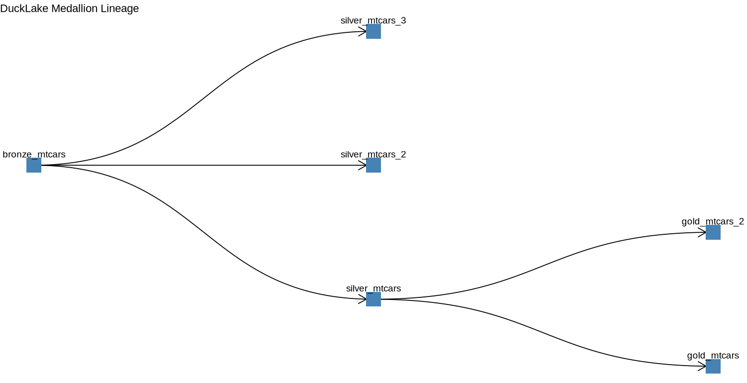
library(igraph)
library(ggraph)

edges <- dbGetQuery(con, "SELECT parent_table AS from_table, child_table AS to_table FROM ducklake_lineage")
g <- graph_from_data_frame(edges, directed = TRUE)

ggraph(g, layout = "tree") +
  geom_edge_diagonal(arrow = arrow(length = unit(4, 'mm')), end_cap = circle(3, 'mm')) +
  geom_node_point(shape = 15, size = 8, color = "steelblue", fill = "lightblue") +
  geom_node_text(aes(label = name), vjust = -1.2, size = 4) +
  coord_flip() +
  scale_y_reverse() +
  theme_void() +
  ggtitle("DuckLake Medallion Lineage")
This plot could be part of a Quarto report or a Shiny app with some interactivity to keep track of the transformations that happen to the data you are managing.
Could be improved upon. See Databricks Unity Catalog view
Python
Requires {duckdb} > 1.3.0
Basic within Quarto
import duckdb con = duckdb.connect(database = ":memory:") con.sql("INSTALL ducklake") con.sql( f""" ATTACH 'ducklake:{r.db_file}' AS my_ducklake (READ_ONLY); """) df = con.sql( """ USE my_ducklake; SELECT * FROM stats LIMIT 1000; """ ).to_df() con.close()- r.db_file is a path variable from an R chunk in a Quarto notebook. See R example.
Create Instance
import duckdb from pathlib import Path # Define our working directories DUCKLAKE_FOLDER = Path("../ducklake_basic") ducklake_metadata = DUCKLAKE_FOLDER / "metadata" ducklake_files = DUCKLAKE_FOLDER / "data_files" duckdb.sql("INSTALL ducklake") duckdb.sql(f""" ATTACH 'ducklake:{ducklake_metadata}' AS ducklake_basic_db (DATA_PATH '{ducklake_files}'); USE ducklake_basic_db; """)/concantenate the pathsATTACHhas the paths for the data files and the metadata filesUSEsets this db as the default
Create Schema and Tables
duckdb.sql("""
    CREATE SCHEMA IF NOT EXISTS retail_sales;
    USE retail_sales;
    """)

duckdb.sql("""
    CREATE TABLE IF NOT EXISTS customer (
        customer_id INTEGER NOT NULL,
        first_name VARCHAR NOT NULL,
        last_name VARCHAR NOT NULL,
        date_joined DATE NOT NULL
    );
    """)
duckdb.sql("""
    CREATE TABLE IF NOT EXISTS orders (
        order_id INTEGER NOT NULL,
        customer_id INTEGER NOT NULL,
        order_date DATE NOT NULL,
        product_id INTEGER NOT NULL,
        product_name VARCHAR NOT NULL,
        amount DECIMAL(10, 2) NOT NULL
    );
    """)
Insert
duckdb.sql("""
    INSERT INTO customer (customer_id, first_name, last_name, date_joined) VALUES
    (1, 'Jane', 'Dunbar', '2023-01-11'),
    (2, 'Jimmy', 'Smith', '2024-08-26'),
    (3, 'Alice', 'Johnston', '2023-05-05');
""")
duckdb.sql("""
    INSERT INTO orders (order_id, customer_id, product_id, product_name, order_date, amount) VALUES
    (1, 1, 101, 'Widget A', '2023-01-15', 19.50),
    (2, 1, 102, 'Widget B', '2023-01-20', 29.99),
    (3, 3, 103, 'Widget A', '2023-02-10', 19.50);
""")
Check file structure
duckdb.sql(f""" FROM glob('{ducklake_files}/*'); """) #> ┌────────────────────────────────────────────────────────────────────────────────────┐ #> │ file │ #> │ varchar │ #> ├────────────────────────────────────────────────────────────────────────────────────┤ #> │ ../ducklake_basic/data_files/ducklake-01978495-e183-7763-bf40-d9a85988eed9.parquet │ #> └────────────────────────────────────────────────────────────────────────────────────┘- Flat file structure with UUID-based naming which is quite different from hierarchical folder structures used by other lakehouse formats
Fetch a parquet file and read it
# Extract the parquet file name
parquet_file = duckdb.sql(f"""
    SELECT file FROM glob('{ducklake_files}/*.parquet') LIMIT 1;
    """).fetchone()[0]

# Inspect the file contents
duckdb.sql(f"""
    SELECT * FROM read_parquet('{parquet_file}');
    """)
#> ┌─────────────┬────────────┬───────────┬─────────────┐
#> │ customer_id │ first_name │ last_name │ date_joined │
#> │    int32    │  varchar   │  varchar  │    date     │
#> ├─────────────┼────────────┼───────────┼─────────────┤
#> │           1 │ Jane       │ Dunbar    │ 2023-01-11  │
#> │           2 │ Jimmy      │ Smith     │ 2024-08-26  │
#> │           3 │ Alice      │ Johnston  │ 2023-05-05  │
#> └─────────────┴────────────┴───────────┴─────────────┘
View snapshot
duckdb.sql("""
    SELECT * FROM ducklake_snapshots('ducklake_basic_db');
    """)
#> ┌─────────────┬────────────────────────────┬────────────────┬─────────────────────────────────────────────────────────────────────────┐
#> │ snapshot_id │       snapshot_time        │ schema_version │                                 changes                                 │
#> │    int64    │  timestamp with time zone  │     int64      │                         map(varchar, varchar[])                         │
#> ├─────────────┼────────────────────────────┼────────────────┼─────────────────────────────────────────────────────────────────────────┤
#> │           0 │ 2025-06-18 19:48:24.41+00  │              0 │ {schemas_created=[main]}                                                │
#> │           1 │ 2025-06-18 19:48:24.489+00 │              1 │ {schemas_created=[retail_sales]}                                        │
#> │           2 │ 2025-06-18 19:48:24.533+00 │              2 │ {tables_created=[retail_sales.customer]}                                │
#> │           3 │ 2025-06-18 19:48:24.554+00 │              2 │ {tables_inserted_into=[2]}                                              │
#> └─────────────┴────────────────────────────┴────────────────┴─────────────────────────────────────────────────────────────────────────┘
Every operation in DuckLake creates a snapshot — a point-in-time view of the database state
Interpretation
- Snapshot 0: Default
mainschema created - Snapshot 1: Our
retail_salesschema created - Snapshot 2: Customer table created
- Snapshot 3: Data inserted into the table
- Snapshot 0: Default
Update and Delete
duckdb.sql(""" UPDATE customer SET first_name = 'Alice', last_name = 'Fraser' WHERE customer_id = 3; """) duckdb.sql(""" DELETE FROM customer WHERE customer_id = 2; """)- DuckLake creates separate “delete files” that reference the original data files and specify which rows should be considered deleted. This approach allows for efficient deletes without rewriting large data files.
Time Travel
- 1
- Query data as it was prior to the latest action
- 2
- Query data as it was prior to the 2 latest actions
Multitable Transaction
duckdb.sql("""
    BEGIN TRANSACTION;
    INSERT INTO customer (customer_id, first_name, last_name, date_joined) VALUES
    (4, 'Bob', 'Brown', '2023-03-01');
    INSERT INTO orders (order_id, customer_id, product_id, product_name, order_date, amount) VALUES
    (4, 4, 104, 'Widget B', '2023-03-05', 29.99),
    (5, 4, 105, 'Widget C', '2023-02-15', 59.99),
    (6, 4, 106, 'Widget A', '2023-01-25', 19.50);
    COMMIT;
""")
This entire operation — adding a customer and three orders — appears as a single snapshot in our change history.
If any part of the transaction had failed, the entire operation would have been rolled back, ensuring data consistency.
Multi-table transactions ensure your data maintains integrity across related tables, something that’s challenging or impossible with table-level formats.
View Changes Due to Latest Transaction
duckdb.sql(f"""
    SELECT * FROM ducklake_table_changes('ducklake_basic_db', 'retail_sales', 'customer', {max_snapshot_id}, {max_snapshot_id})
    ORDER BY snapshot_id;
    """)
#> ┌─────────────┬───────┬─────────────┬─────────────┬────────────┬───────────┬─────────────┬─────────┐
#> │ snapshot_id │ rowid │ change_type │ customer_id │ first_name │ last_name │ date_joined │  email  │
#> │    int64    │ int64 │   varchar   │    int32    │  varchar   │  varchar  │    date     │ varchar │
#> ├─────────────┼───────┼─────────────┼─────────────┼────────────┼───────────┼─────────────┼─────────┤
#> │           9 │     6 │ insert      │           4 │ Bob        │ Brown     │ 2023-03-01  │ NULL    │
#> └─────────────┴───────┴─────────────┴─────────────┴────────────┴───────────┴─────────────┴─────────┘