Troubleshooting HMC
Divergent Transitions
- “divergent transitions after warmup”
- See Taming Divergences in Stan Models and Identifying non-identifiability
- See Statistical Rethinking >> Ch.9 MCMC >> Issues
- Divergent Transition - A rejected proposed parameter value in the posterior during the sampling process
- Too many DTs could indicate a poor exploration of the posterior by the sampling algorithm and possibly biased estimates.
- If the DTs are happening in the same region of the posterior then that region isn’t being sampled by the HMC algorithm
- If there are “steep” areas in the posterior, these areas can break the sampling process resulting in a “bad” proposed parameter value.
- Too many DTs could indicate a poor exploration of the posterior by the sampling algorithm and possibly biased estimates.
- Solutions
- Adjust priors from flat to weakly informative
- Need more data
- Increase adapt_delta closer to 1 (default: 0.8)
- Reparameterize the model
Chains Not Mixing
Misc
Minor Issues
Priors on some parameters are weak or nonexistent or the data are too weak to identify all the parameters in the model.
- Signs: Chains are exploring extreme regions of the parameter space. Check out the y-axis range in trace and see how high or low the values are.
- Examples: elasticity parameters of -20 or people with 8 kg livers
Chains are flat-lining sometimes (source)
- Solution: Rescaling predictors to 0-1 range and setting intial values at 0
Coding mistake
- Stan examples:
- You can forget to use a log link or set a prior using variance instead sd
- Array indices and for loops don’t match
- Stan examples:
Multi-Modal Posterior
- Minor modes in the tails of the posterior distribution
- Your posterior is multimodal and all but one of the modes have near-zero mass
- When the posterior distribution is multimodal, it means that there are multiple distinct regions of high probability density, separated by regions of low probability density. This can lead to poor mixing of the MCMC chains, as the chains may get stuck in one of the modes and have difficulty exploring the other modes.
- Signs: different chains will cluster in different places
Solutions
- Pathfinder
- Paper, Github
- Gets rid of lots of these minor modes automatically
- A Variational Inference (VI) method that locates approximations to the target density along a quasi-Newton optimization path. Starting from a random initialization in the tail of the posterior distribution, the quasi-Newton optimization trajectory can quickly move from the tail, through the body of the distribution, to a mode or pole.
- Variational inference searches for a tractable approximate distribution that minimizes Kullback-Leibler (KL) divergence to the posterior and is typically faster than Monte Carlo sampling.
- Use starting values near the main mode
- {brms} init argument (See Statistical Rethinking >> Ch 4)
- Can also be used in general cases where you’re getting bad mixing from you chains
- e.g. divergent transitions, large numbers of transitions, high R-hat values, and/or very low effective sample size estimates
- Example:
Diagnose Issue: Check the intercept warm-up (For real-world models, it’s good to look at the trace plots for all major model parameters)
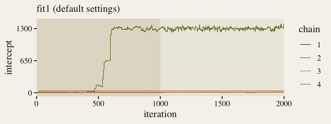
geom_trace <- function(subtitle = NULL, xlab = "iteration", xbreaks = 0:4 * 500) { list( annotate(geom = "rect", xmin = 0, xmax = 1000, ymin = -Inf, ymax = Inf, fill = fk[16], alpha = 1/2, size = 0), geom_line(size = 1/3), scale_color_manual(values = fk[c(3, 8, 27, 31)]), scale_x_continuous(xlab, breaks = xbreaks, expand = c(0, 0)), labs(subtitle = subtitle), theme(panel.grid = element_blank()) ) } p1 <- ggmcmc::ggs(fit1, burnin = TRUE) %>% filter(Parameter == "b_Intercept") %>% mutate(chain = factor(Chain), intercept = value) %>% ggplot(aes(x = Iteration, y = intercept, color = chain)) + geom_trace(subtitle = "fit1 (default settings)") + scale_y_continuous(breaks = c(0, 650, 1300), limits = c(NA, 1430)) p1- One of our chains eventually made its way to the posterior, three out of the four stagnated near their starting values (lines near zero).
Set starting values manually. Same values to all 4 chains
.png)
inits <- list(
  Intercept = 1300,
  sigma    = 150,
  beta      = 520
)
list_of_inits <- list(inits, inits, inits, inits)
fit2 <- brm(
  data = dat,
  family = exgaussian(),
  formula = rt ~ 1 + (1 | id),
  cores = 4, seed = 1,
  inits = list_of_inits
)
Much mo’ better, but not evidence of chain convergence since all started at the same value
No practical for large models with many parameters
Set starting values (somewhat) randomly by function
.png)
set_inits <- function(seed = 1) {
  set.seed(seed)
  list(
    # posterior for the intercept often looks gaussian
    Intercept = rnorm(n = 1, mean = 1300, sd = 100),
    # posteriors for sigma and beta need to nonnegative (alt:rgamma)
    sigma    = runif(n = 1, min = 100, max = 200),
    beta      = runif(n = 1, min = 450, max = 550)
  )
}

list_of_inits <- list(
  # different seed values will return different results
  set_inits(seed = 1),
  set_inits(seed = 2),
  set_inits(seed = 3),
  set_inits(seed = 4)
)
Chains are mixing and evidence of convergence since we started at different starting values
Need to also check sigma and beta
- Fit multiple models and average predictions (stacking). Don’t fully understand but this is from a section 5.6 of Gelman’s Bayesian Workflow paper
- “Divide the model into pieces by introducing a strong mixture prior and then fitting the model separately given each of the components of the prior. Other times the problem can be addressed using strong priors that have the effect of ruling out some of the possible modes”
- Reparameterize the Model
- Think this had to do with Divergent Transitions
- Signs: You have coefficients like 0.000002
- Solutions:
- Use variables that have been log transformed or scaled (e.g. per million). For some reason, itt’s difficult for the sampler when parameters values are on vastly different scales.
- Reparameterize to “unit scale”
- I think scale in “unit scale” refers to scale as a distribution parameter like sd is the scale parameter in a Normal distribution, and “unit scale” is scale = 1 (e.g. sd = 1 in standardization). But there’s more to this, and I haven’t read S.R. ch 13 yet
- Common (misguided?) Solutions
- Increase iterations
- Tweak adapt_delta and max_treedepth parameters to make it explore the space more carefully
- Other
- Sequential Monte Carlo (SMC) is a potential solution multimodal posterior problem (Stan’s NUTS sampler may already do this to some extent. See Ch. 9 Statistical Rethinking)
- Algorithm details - https://docs.pymc.io/notebooks/SMC2_gaussians.html?highlight=smc
- Sequential Monte Carlo (SMC) is a potential solution multimodal posterior problem (Stan’s NUTS sampler may already do this to some extent. See Ch. 9 Statistical Rethinking)
Reparameterization
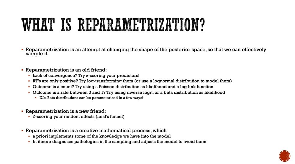
Note: “RT’s” in the image is probably refering to a response variable (e.g. Response Time, Reaction Time, etc.)
Used to help solve HMC issues where sampling behaviour can suffer in the presence of difficult posterior geometries: for instance, when the posterior has heavy tails or nonlinear correlations between parameters
Misc
- Resources
- See Stan User Guide (newer version)
- See Ch 13.4 in Statistical Rethinking
- Also see {makemypriors} in Bayes, Priors >> Misc >> Packages - Recommended in the Thread below as method for handling the same issues that reparameterization solves.
- Notes from Thread
- In the paper, Strategies for fitting nonlinear ecological models in R, AD Model Builder, and BUGS, it suggests scaling; eliminating correlation; making contours elliptical.(?)
- Gamma from {shape,scale} to {log-mean, log-shape} is often good.
- Resources
Parameters with distributions such as cauchy, student-t, normal, or any distribution in the location-scale family are good reparameterization candidates
Neal’s Funnel
- Technique for efficiently sampling random effects or latent variables in hierarchical Bayesian models.
- Z-Scores Random Effects
Example: McElreath
\[ \begin{align} &x \sim \text{Exponential}(\lambda) \\ &\quad\quad\text{-same as-} \\ &z \sim \text{Exponential(1)} \\ &x = \frac{z}{\lambda} \end{align} \]
- Factoring out scale parameters
Non-Centered Parameterizations
Briefly, this means restating the target distribution (i.e. the posterior) in terms of parameters which do not have the same hierarchical dependence structures as in the original parameterization, thereby inducing a posterior geometry more amenable to HMC.
The parameters of interest are then recovered as deterministic functions of the ones actually sampled.