Multilevel, Longitudinal
Misc
- Also see Mixed Effects, General >> Considerations >> Variable Assignment
- Need to figure out if
- There’s significant within-unit variation. If so, then FE model will likely be the best model
- Article with simulated data showed that within variation around sd < 0.5 didn’t detect the effect of explanatory variable but ymmv (depends on # of units, observations per unit, N)
- There’s significant between-unit variation. If so, then RE model will likely be the best model
- There’s significant within-unit variation. If so, then FE model will likely be the best model
- Packages
Multilevel
- Misc
- Also see Regression, Ordinal >> EDA >> Crosstabs
- Is my data clustered?
- Separate variables into levels
- Level One: Variables measured at the most frequently occurring observational unit
- i.e. Variables that (for the most part) have different values for each row
- i.e. Vary for each repeated measure of a subject and vary between subjects
- Level Two: Variables measured on larger observational units
- i.e. Constant for each repeated measure of a subject but vary between each subject
- Level One: Variables measured at the most frequently occurring observational unit
Univariate
- Level 1 and Level 2
- Group-level correlation or autocorrelation in variables can mislead or obscure patterns
- If level 2 variable categories are pretty well balanced and there’s sufficient data, then plotting means can remove the correlation affect in the plot
- Continuous
- Looking at the skew, median/mean, bimodal or not
- Example:
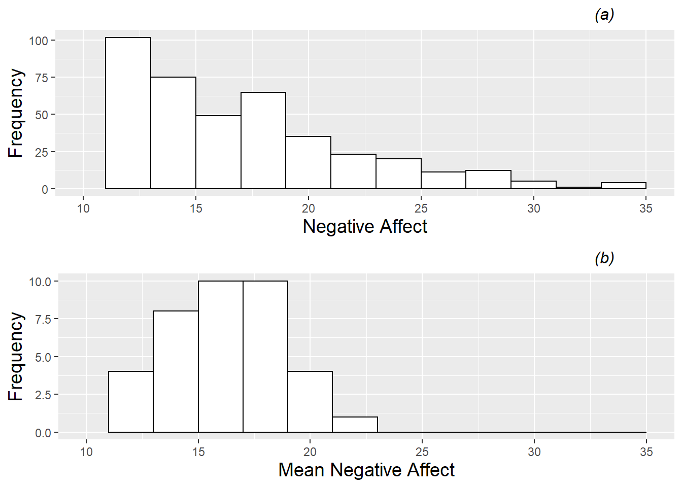
- (Top) Each observation is plotted as if each observation is independent of the other
- * Ignores dependency (via repeated measures)
- (Bottom) Means for each subject or case or other level of a random variable
- * Removes dependency
- Interpretation: Right skew remains in both plots but plot 1’s decrease is smoother than plot 2’s
- (Top) Each observation is plotted as if each observation is independent of the other
- Categorical
- Calculate proportions of each category and noting trends (ordinal variables) or severe imbalances
- Group-level correlation or autocorrelation in variables can mislead or obscure patterns
Bivariate
- Questions
- Is there is a general trend suggesting that as the covariate increases the response either increases or decreases (trend)
- Do subjects at certain levels of the covariate tend to have similar mean values of the response (low variability)
- Is the variation in the response at different levels of the covariate (unequal variability)
- Me: Comparison between plots that take into account dependency and the same plot that doesn’t
- Trend in plot that ignores dependency but no trend in plot that removes dependency
- May indicate within-subject variation
- No trend in plot that ignores dependency but trend in plot that removes dependency
- May indicate between-subject variation
- Trend in plot that ignores dependency but no trend in plot that removes dependency
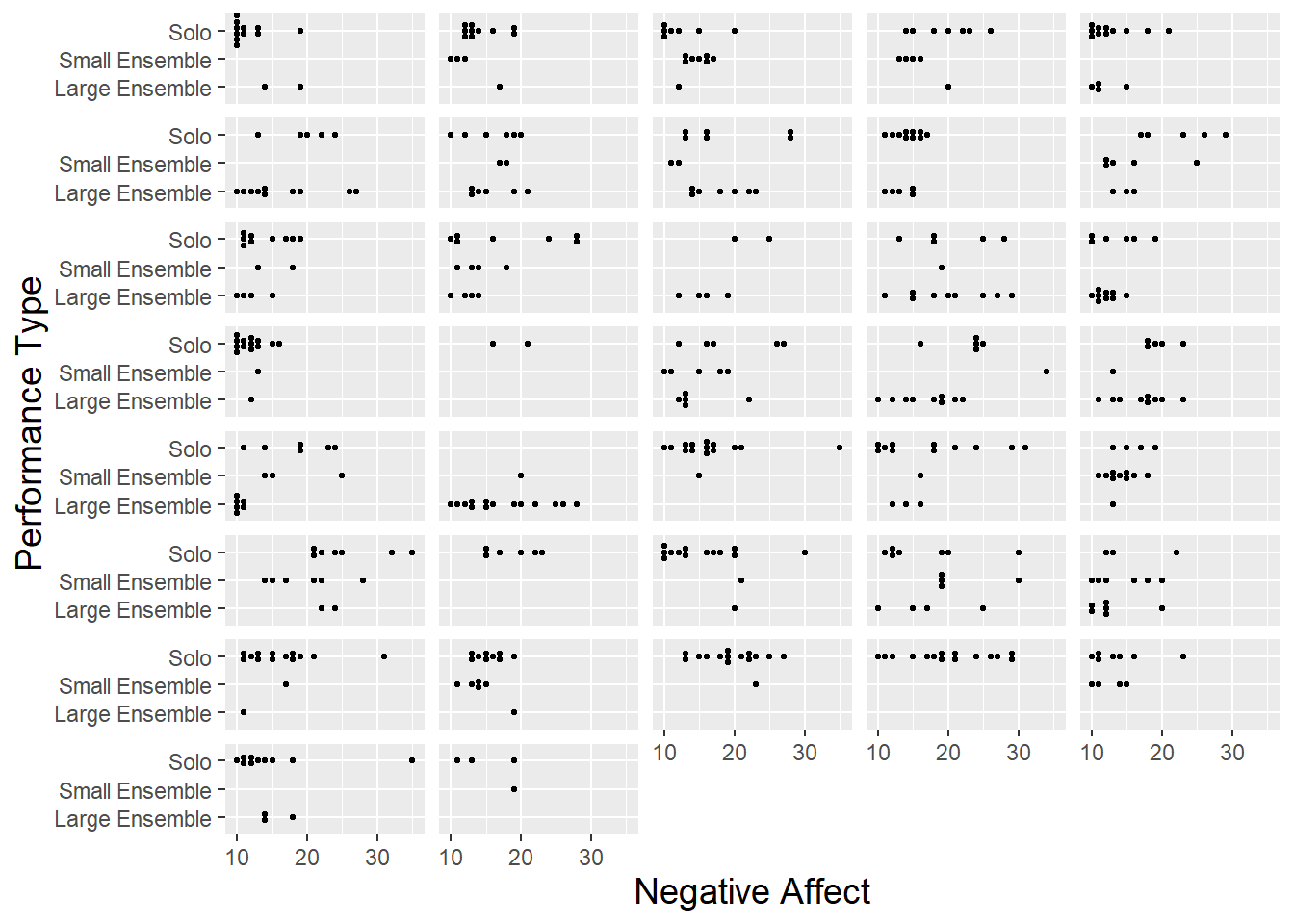
- Boxplots (Categorical)
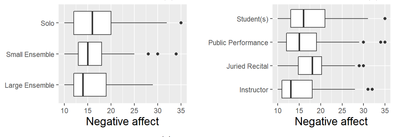
- Level 1 categorical covariates (y-axis) vs continuous outcome (x-axis)
- * Ignores dependency (via repeated measures)
- Interpretation
- Left: ordinal covariate, medians are close and boxes pretty much contained within each other but there might be a trend
- Right: Looks like some decent variation between categories
- Mean outcome (per subject) vs covariate

- * Removes dependency
- Interpretation: looks like some decent variation between categories
- Scatter (Continuous)
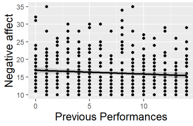
- Level 1 continuous covariate (x-axis) vs continuous outcome (y-axis)
- * Ignores dependency (via repeated measures)
- Actually a discrete covariate being treated as continuous the fact that does seem to be a small trend is what’s important
- Mean outcome (per subject) vs covariate
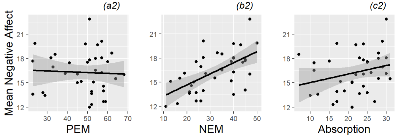
- * Removes dependency
- Interpretation: PEM not showing much of an correlation if any
- Facetting previous plots by subject
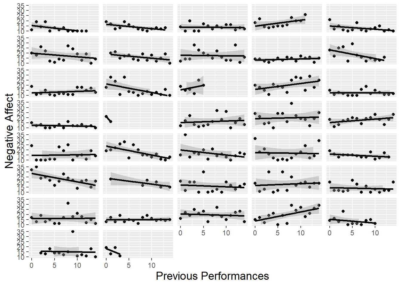
- Left
- Mostly downward trends but some upward trends
- Useful for prior formulation
- Gives an idea about the uncertainty of the slope of this variable
- Right
- Scarcity of points for some categories makes boxplots a bad idea
- Difficult to spot any trends
- * Removes dependency
- Left
Trivariate
Scatter, color by random variable
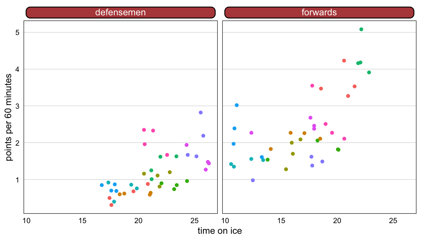
- Variables
- “points per 60 min” (outcome)
- “time on ice” (fixed effect)
- facetted by “position” (fixed effect)
- colored by “player” (potential random variable)
- Interpretation
- Theres does seem to be clustering by “player” therefore a mixed effects model might be a good choice.
- Variables
Scatter with linear smooths (link)
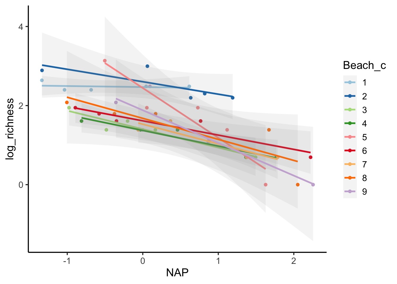
theme_set(theme_classic(base_size = 14)) ggplot(d, aes(x = NAP, y = log_richness, color = Beach_c)) + geom_point() + stat_smooth(method = "lm", alpha = 0.1) + scale_color_brewer(palette = "Paired")- Shows the varying slopes and some varying intercepts (but an overall trend) by random variable, Beach_c
Null Model (aka random intercept-only model)
m0 <- lmer(pp60 ~ 1 + (1 | player), data = df) jtools::summ(m0) GROUPING VARIABLES GROUP # GROUPS ICC player 20 0.89- ICC > 0.1 is generally accepted as the minimal threshold for justifying the use of Mixed Effects model (See ICC section)
Longitudinal
- Misc
- Repeated measures that have a sequential or time component
- Packages:
- {brolgar}
- Efficiently explore raw longitudinal data
- Calculate features (summaries) for individuals
- Evaluate diagnostics of statistical models
- {gglinedensity} - Provides a “derived density visualisation (that) allows users both to see the aggregate trends of multiple (time) series and to identify anomalous extrema.”
- {brolgar}
Univariate
- Continuous Outcome vs. Time
- Facetted by Observational Unit (e.g. school)
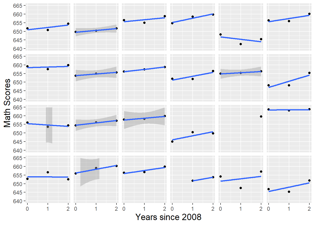
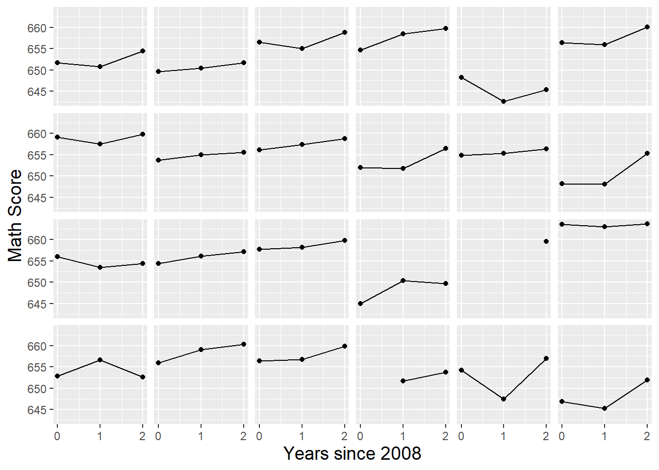
- Linear Fit and Line Chart
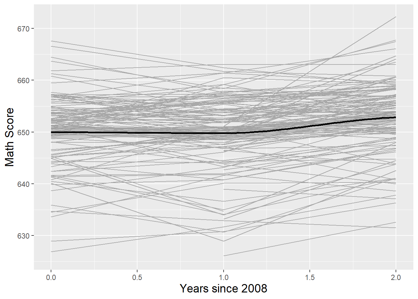
- Spaghetti
- Facetted by Observational Unit (e.g. school)
Bivariate
Bold line is the overall fit with LOESS
Continuous Outcome vs Time
- Facetted by Categorical
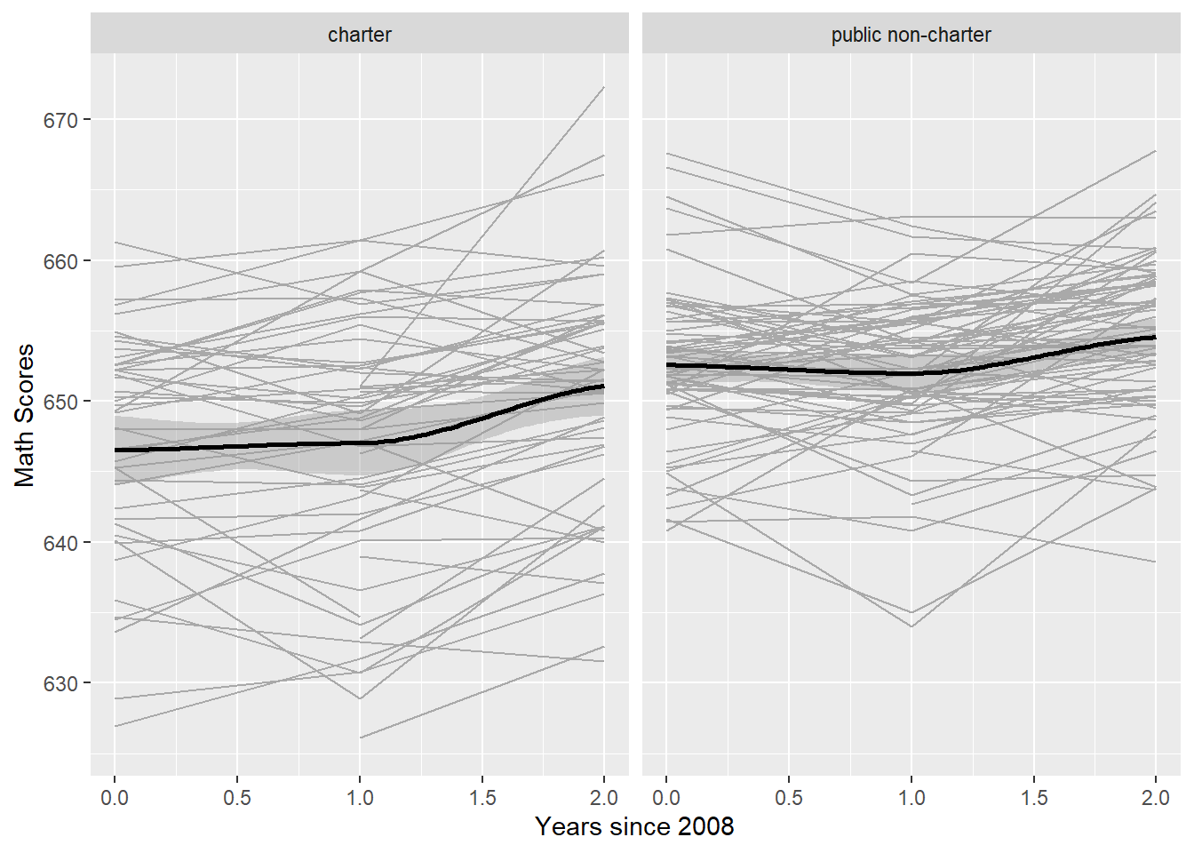
- Facetted by Binned Continuous
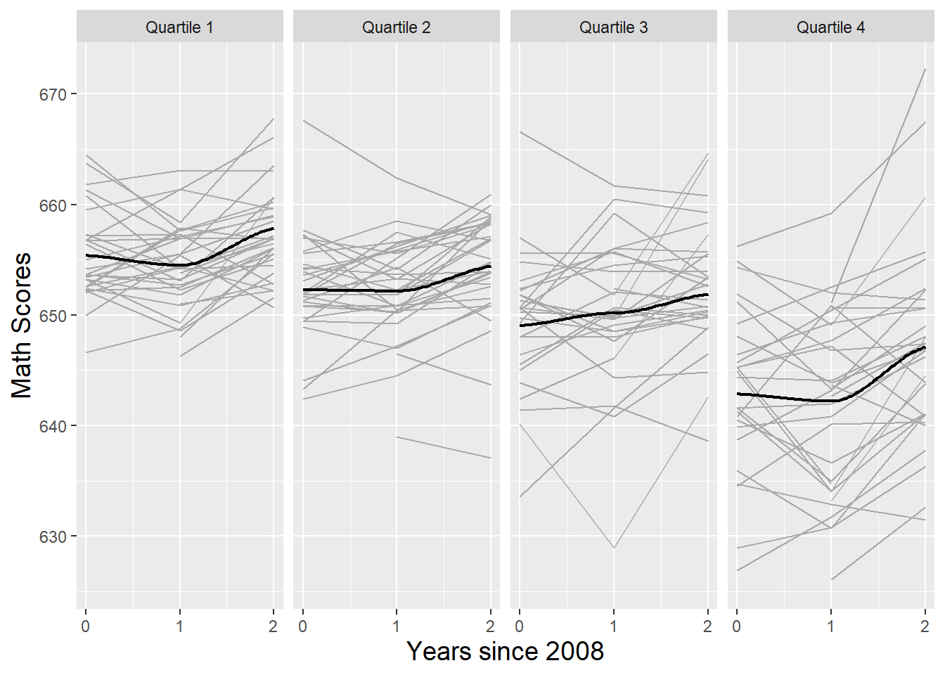
- Facetted by Categorical
Time Endpoints
.png)
- “School Type” is a categorical, level 2 variable and “Math Score” is the numeric outcome
- Looking for change from the initial measurement to the final measurement
Linear parameters
- Fit a linear regression for each subject/unit with its repeated measurements
- See univariate >> numerical outcome vs. time >> Facetted by observational unit >> (left) linear fit
- Advantages
- Each unit’s/subject’s data points can be summarized with two summary statistics—an intercept and a slope
- Bigger advantage when there are more observations over time per unit/subject
- Seems like a good way for using empirical bayes (i.e. use these distributions for prior specifications)
- Each unit’s/subject’s data points can be summarized with two summary statistics—an intercept and a slope
- Disadvantages
- Slopes cannot be estimated for those units/subjects with just a single observation
- R-squared values cannot be calculated for those units/subjects with no variability in test scores during the time period
- R-squared values must be 1 for those units/subjects with only two test scores.
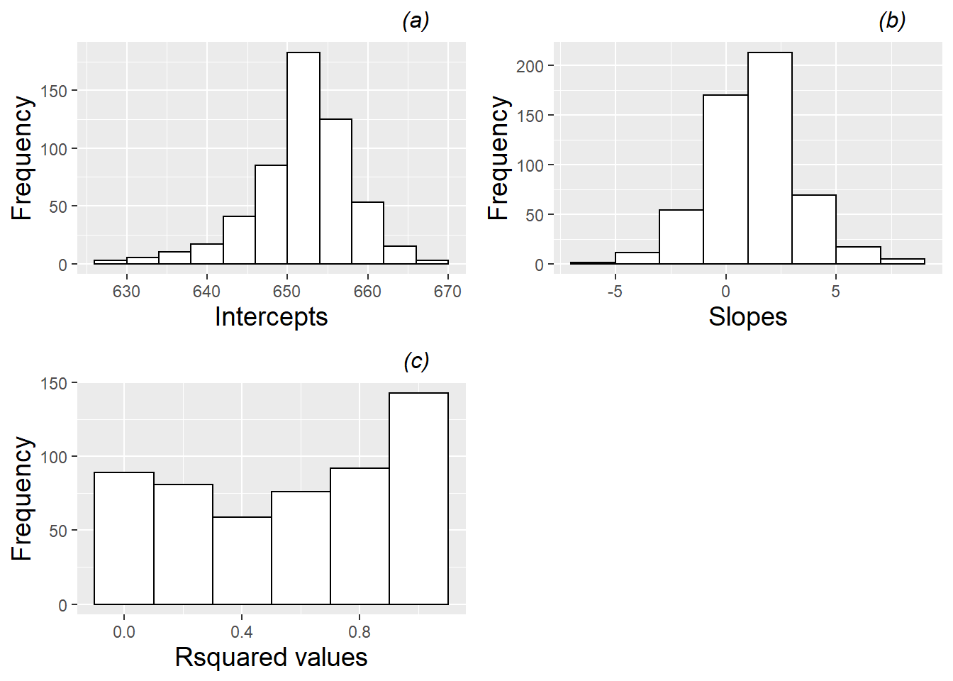
- Summary Statistics
- Mean and SD for intercepts and slopes
- Univariate
- \(y_t = \beta_0 + \beta_1 t + \epsilon_t\)
- \(t\) is the time variable (aka trend)
- Parameter Distributions
- Correlation
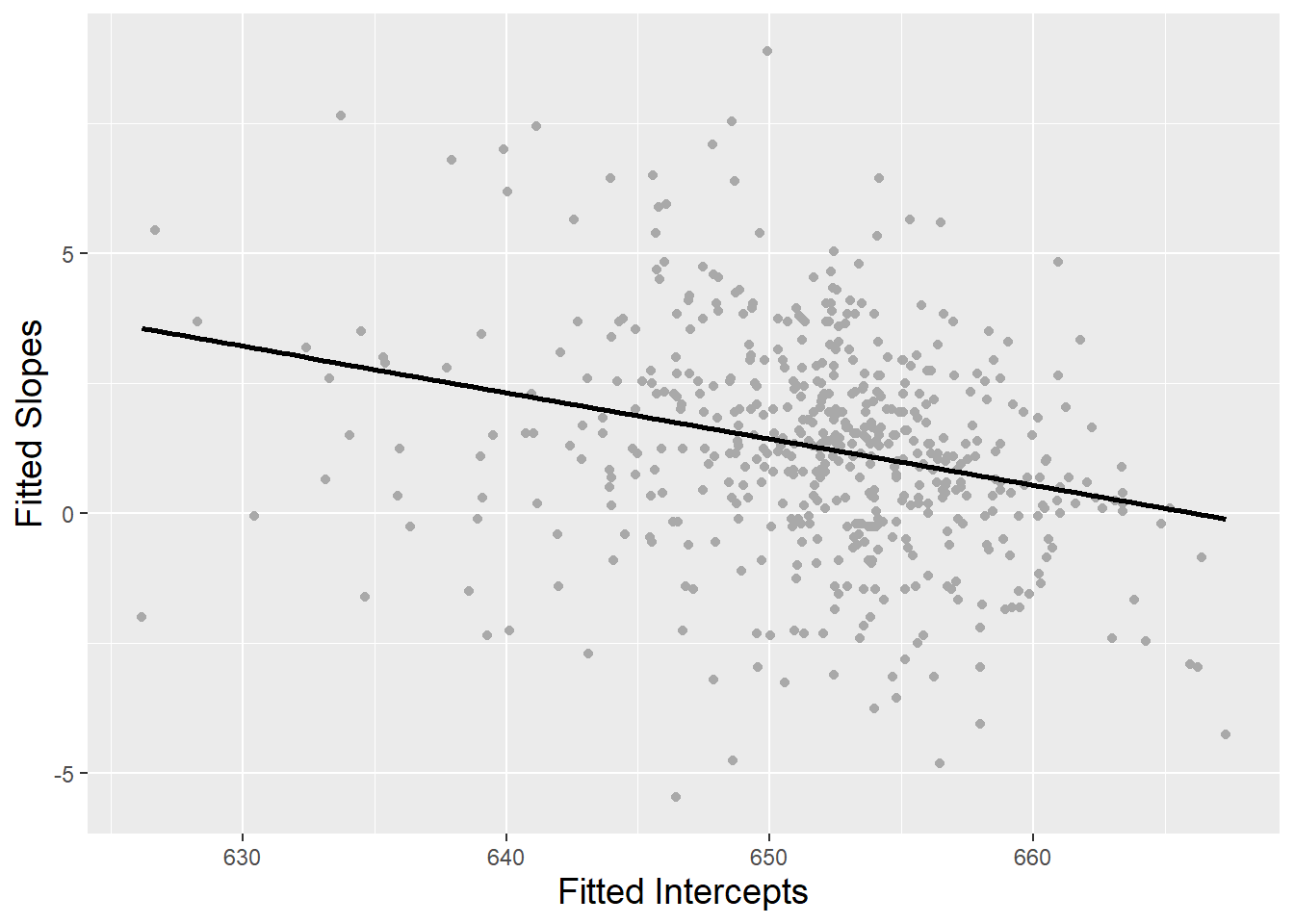
- Lower intitial values (intercepts) show the greatest growth (slopes) over time
- Correlation = -0.32
- \(y_t = \beta_0 + \beta_1 t + \epsilon_t\)
- Bivariate
- Process
- Filter data by Level 2 variable
- For each category of the Level 2 variable, fit a regression, yt = β0 + β1t + εt, for each unit/subject.
- Aggregate results
- Parameter Distributions
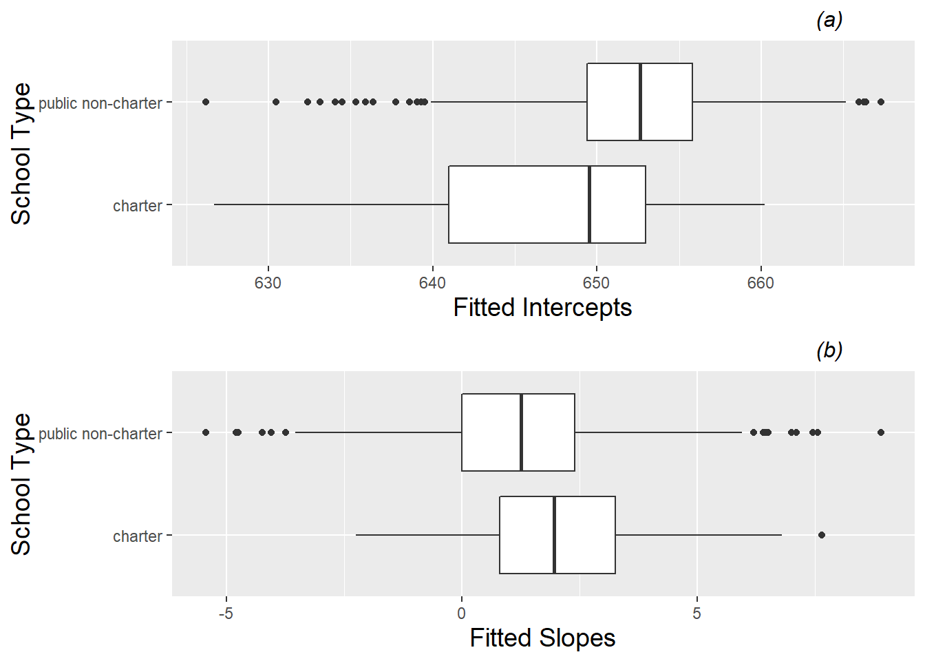
- “School Type” is a Level 2, binary variable
- Process