Optimization

Misc

A while loop is faster than a recursive function
ungroup before performing calculations in mutate or summarize when that calculation doesn’t need to be performed within-group (i.e. per factor level)
String functions
- “fixed” searches, fixed = TRUE are fastest overall
  - Searches involving fixed strings (e.g. “banana”) that don’t require regular expressions
- PCRE2, perl = TRUE , is fastest for regular expressions

Adding Rows to a Matrix (link, link)

rbind is very slow and cbind + t() isn’t much better

frbind <- function(n) {
    res <- vector()
    for (i in 1:n) {
        res <- rbind(res, runif(n))
    }
    res
}
fcbind <- function(n) {
    res <- vector()
    for (i in 1:n) {
        res <- cbind(res, runif(n))
    }
    t(res)
}

Add rows to a list then combine into a matrix

# grow list which is converted to a matrix at the end.
flist <- function(n) {
    res <- list()
    for (i in 1:n) {
        res[[length(res) + 1]] <- runif(n)
    }
    do.call(rbind, res)
}
flist2 <- function(n) {
    res <- list()
    for (i in 1:n) {
        res[[length(res) + 1]] <- runif(n)
    }
    len <- length(res)
    res <- res |> purrr::list_c()
    dim(res) <- c(len, len)
    res
}

list_c uses C under the hood and might be faster on larger matrices.

Benchmarking

Misc
- Mastering Software Development in R, Ch. 2.71
{bench}
- Misc
  - Automatically checks that each approach gives the same output, so that you don’t mistakenly compare apples and oranges
  - bench::mark creates a very large output object. The one in Vectorization Workflows >> Example 1 was 400MB. RStudio View locked up when I tried to look at it. There are large dataframes nested within the memory and result columns. Setting the option memory = FALSE only decreases the size of the object very little. Compilation of this object will take a minute or two after the benchmark has technically finished.
- Example: Basic
```
res <-
  bench::mark(
    approach_1 = Reduce(sum, numbers),
    approach_2 = sum(unlist(numbers))
  )

res %>% select(expression, median)

#> # A tibble: 2 × 2
#>  expression  median
#>  <bch:expr> <bch:tm>
#> 1 approach_1  2.25µs
#> 2 approach_2 491.97ns
```

{microbenchmark}

Example: Basic

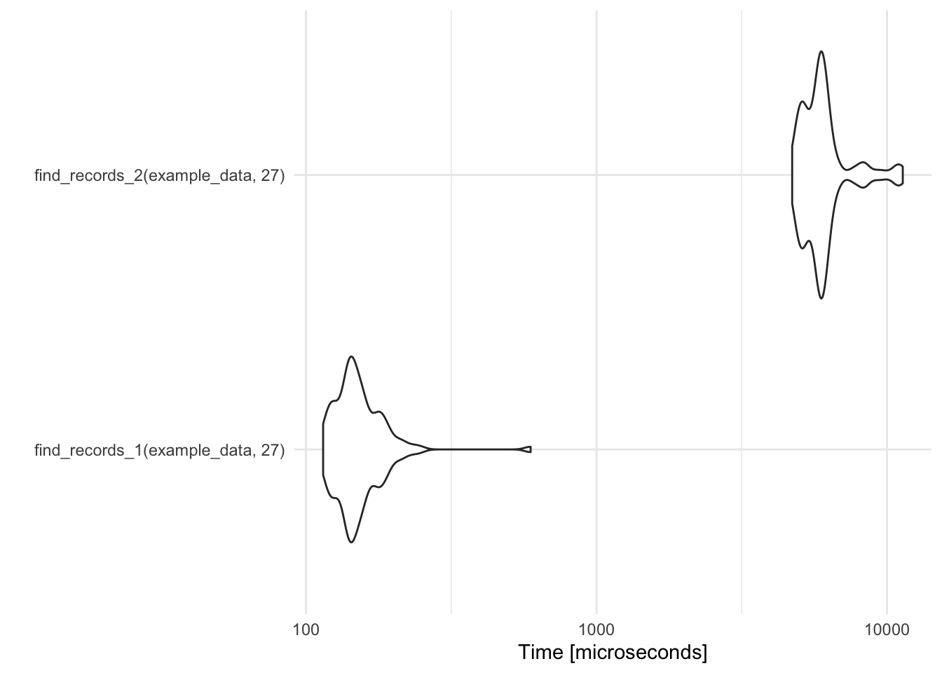
record_temp_perf <- microbenchmark(find_records_1(example_data, 27), 
                                  find_records_2(example_data, 27))
record_temp_perf

## Unit: microseconds
##                              expr      min      lq      mean  median      uq
##  find_records_1(example_data, 27)  114.574  136.680  156.1812  146.132  163.676
##  find_records_2(example_data, 27) 4717.407 5271.877 6113.5087 5867.701 6167.709
##        max neval
##    593.461  100
##  11334.064  100

library(ggplot2)
autoplot(record_temp_perf)

Default: 100 iterations
Times are given in a reasonable unit, based on the observed profiling times (units are given in microseconds in this case).
Output
- min - min time
- lq - lower quartile
- mean, median
- uq - upper quartile
- max - max time

Profiling

Misc
- Resources
  - Mastering Software Development in R, Ch. 2.72
  - Advanced R, Ch. 23
  - Repo of R profiling tools
- Packages
  - {profvis} - Interactive Visualizations for Profiling R Code
  - {profmem}: Simple Memory Profiling for R
  - {syrup}: Provide measures of memory and CPU usage for parallel R code
  - {memuse} - An R package for memory estimation.
    - Tools for estimating the size of a matrix (that doesn’t exist), showing the size of an existing object in a nicer way than object.size(). It also has tools for showing how much memory the current R process is consuming, how much ram is available on the system, and more.
{profvis}
- Notes from Unveiling Bottlenecks (Part 2): A Deep Dive into Profiling Tools
- Features
  - Vertical Bars: Each vertical bar in the flame graph represents a function call stack in your code. The height of the bar indicates the depth of the call stack, with the top-most bar representing the outermost function call.
  - Colors: Different colors are used to distinguish between different functions or code blocks. Colors often depict different code categories (e.g., user code, Shiny functions, R base functions).
  - Width of Bars: The width of each bar corresponds to the amount of time spent executing the function. Wider bars indicate that more time was spent in that particular function.
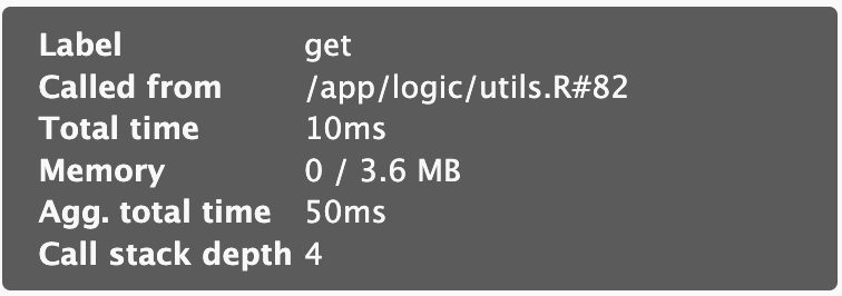
  - Clicking on Bars: Clicking on a bar representing a function call often reveals additional information such as the function name, self time (time spent within the function), and total time (including time spent in functions it calls).
  - Clicking on Cells: Single click on cell will move you to the specific function, double click on cell will redirect you to code editor in a separate window, additionally it will expand the bar to provide you a more clear view.
  - Data Tab: A hierarchical table showing the profile in a top-down manner. Allows you to check the Memory and Time columns for resource allocation insights.
- Analyzing the Flame Graph
  - Identifying Bottlenecks: Look for sections with the widest bars. These represent functions that consume the most execution time and are potential bottlenecks.
  - Understanding Call Stack: Trace the path downwards from the top to identify the sequence of function calls leading to the bottleneck.
  - Zooming In: Use interactive features to zoom in on specific sections for a closer look at nested function calls.
  - Comparing Runs: You can compare flame graphs from different app versions to identify performance improvements or regressions.
- Interpreting the Information
  - Time Spent in Functions: The width of a bar at a specific level reveals the time spent executing that particular function.
  - Self Time vs. Total Time: Some profvis implementations differentiate between “self time” (time spent within the function itself) and “total time” (including time spent in functions it calls). This helps identify functions that contribute significantly to bottlenecks through nested calls.
  - Code Optimization: By focusing on functions with the widest bars, you can prioritize optimization efforts by re-factoring code, leveraging vectorization, or exploring alternative algorithms.
- Example: Basic
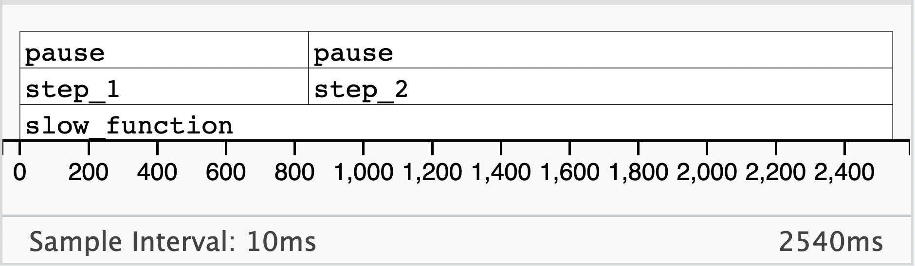
```
step_1 <- function() {
  pause(1)
}
step_2 <- function() {
  pause(2)
}
slow_function <- function() {
  step_1()

  step_2()

  TRUE
}
result <- profvis(slow_function())
result
```
  - Bottom Row: outermost function
  - 2nd Row from the bottom are the functions in the next enviromental layer (e.g. “step_1” and “step_2”)
    - “step_2” takes about 2/3 of the total function execution time or twice the execution time of “step_1”
  - 3rd Row from the bottom (top row) are the functions in each of those other functions
    - “pause” in “step_2” takes about 2/3 of the total function execution time or twice the execution time of “pause” in “step_1”

Python

Benchmarking

{{time}}(built-in module)

import time
start = time.perf_counter()
time.sleep(1) # do work
elapsed = time.perf_counter() - start
print(f'Time {elapsed:0.4}')
#> Time 1.001

Memory Usage

Basic usage for a function
```
from memory_profiler import memory_usage
mem, retval = memory_usage((fn, args, kwargs), retval=True, interval=1e-7)
```
- interval: For very quick operations the function fn might be executed more than once. By setting interval to a value lower than 1e-6, we force it to execute only once.
- retval: Tells the function to return the result of fn.

Non-interactive usage

$ python -m memory_profiler example.py
#> Line #    Mem usage  Increment   Line Contents
#> ==============================================
#>      3                           @profile
#>      4      5.97 MB    0.00 MB   def my_func():
#>      5     13.61 MB    7.64 MB       a = [1] * (10 ** 6)
#>      6    166.20 MB  152.59 MB       b = [2] * (2 * 10 ** 7)
#>      7     13.61 MB -152.59 MB       del b
#>      8     13.61 MB    0.00 MB       return a

Profile decorator

import time
from functools import wraps
from memory_profiler import memory_usage

def profile(fn):
    @wraps(fn)
    def inner(*args, **kwargs):
        fn_kwargs_str = ', '.join(f'{k}={v}' for k, v in kwargs.items())
        print(f'\n{fn.__name__}({fn_kwargs_str})')

        # Measure time
        t = time.perf_counter()
        retval = fn(*args, **kwargs)
        elapsed = time.perf_counter() - t
        print(f'Time   {elapsed:0.4}')

        # Measure memory
        mem, retval = memory_usage((fn, args, kwargs), retval=True, timeout=200, interval=1e-7)

        # Get Peak Memory Usage
        print(f'Memory {max(mem) - min(mem)}')
        return retval

    return inner

@profile
def work(n):
   for i in range(n):
       2 ** n

work(10)
#> work()
#> Time   0.06269
#> Memory 0.0

work(n=10000)
#> work(n=10000)
#> Time   0.3865
#> Memory 0.0234375

Replacements for Tidyverse Functions

Misc
- Notes from: Writing performant code with tidy tools
  - Also provides links to more {vctrs} recipes from their tidymodels github pull requests
- For code that relies on group_by()and sees heavy traffic, see vctrs::list_unchop(), vctrs::vec_chop(), and vctrs::vec_rep_each().

select

bench::mark(
  dplyr = select(mtcars_tbl, hp),
  `[.tbl_df` = mtcars_tbl["hp"]
) %>%
  select(expression, median)
#> # A tibble: 2 × 2
#>  expression  median
#>  <bch:expr> <bch:tm>
#> 1 dplyr      527.01µs
#> 2 [.tbl_df    8.08µs

Winner: base R subsetting

filter

Wres <-
  bench::mark(
    dplyr = filter(mtcars_tbl, hp > 100),
    vctrs = vec_slice(mtcars_tbl, mtcars_tbl$hp > 100),
    `[.tbl_df` = mtcars_tbl[mtcars_tbl$hp > 100, ]
  ) %>%
    select(expression, median)
res
#> # A tibble: 3 × 2
#>  expression  median
#>  <bch:expr> <bch:tm>
#> 1 dplyr      289.93µs
#> 2 vctrs        4.63µs
#> 3 [.tbl_df    23.74µs

Winner: vctrs::vec_slice

mutate

bench::mark(
  dplyr = mutate(mtcars_tbl, year = 1974L),
  `$<-.tbl_df` = {mtcars_tbl$year <- 1974L; mtcars_tbl}
) %>%
  select(expression, median)

#> # A tibble: 2 × 2
#>  expression  median
#>  <bch:expr> <bch:tm>
#> 1 dplyr      302.5µs
#> 2 $<-.tbl_df  12.8µs

Winner: base R assignment

mutate and relocate

bench::mark(
  mutate = mutate(mtcars_tbl, year = 1974L, .after = make_model),
  relocate = relocate(mtcars_tbl, year, .after = make_model),
  `[.tbl_df` = 
      mtcars_tbl[
        c(left_cols, 
          colnames(mtcars_tbl[!colnames(mtcars_tbl) %in% left_cols])
        )
      ],
  check = FALSE
) %>% 
  select(expression, median)

#> # A tibble: 3 × 2
#>  expression  median
#>  <bch:expr> <bch:tm>
#> 1 mutate        1.2ms
#> 2 relocate    804.3µs
#> 3 [.tbl_df    19.1µs

Winner: base R

pull

bench::mark(
  dplyr = pull(mtcars_tbl, hp),
  `$.tbl_df` = mtcars_tbl$hp,
  `[[.tbl_df` = mtcars_tbl[["hp"]]
) %>%
  select(expression, median)

#> # A tibble: 3 × 2
#>  expression  median
#>  <bch:expr> <bch:tm>
#> 1 dplyr      101.19µs
#> 2 $.tbl_df  615.02ns
#> 3 [[.tbl_df    2.25µs

Winner: base R bracket subsetting

bind_*

bench::mark(
  dplyr = bind_rows(mtcars_tbl, mtcars_tbl),
  vctrs = vec_rbind(mtcars_tbl, mtcars_tbl)
) %>%
  select(expression, median)

#> # A tibble: 2 × 2
#>  expression  median
#>  <bch:expr> <bch:tm>
#> 1 dplyr          44µs
#> 2 vctrs        14.3µs

bench::mark(
  dplyr = bind_cols(mtcars_tbl, tbl),
  vctrs = vec_cbind(mtcars_tbl, tbl)
) %>%
  select(expression, median)
#> # A tibble: 2 × 2
#>  expression  median
#>  <bch:expr> <bch:tm>
#> 1 dplyr        60.7µs
#> 2 vctrs        26.2µs

Winners: vctrs::vec_cbind and vctrs::vec_rbind

Create Tibble

bench::mark(
  tibble = tibble(a = 1:2, b = 3:4),
  new_tibble_df_list = new_tibble(df_list(a = 1:2, b = 3:4), nrow = 2),
  new_tibble_list = new_tibble(list(a = 1:2, b = 3:4), nrow = 2)
) %>% 
  select(expression, median)
#> # A tibble: 3 × 2
#>  expression          median
#>  <bch:expr>        <bch:tm>
#> 1 tibble            165.97µs
#> 2 new_tibble_df_list  16.69µs
#> 3 new_tibble_list      4.96µs

Winner: new_tibble_list

Joins

Questions:
- If this join happens multiple times, is it possible to express it as one join and then subset it when needed?
  - i.e. if a join happens inside of a loop but the elements of the join are not indices of the loop, it’s likely possible to pull that join outside of the loop and then vctrs::vec_slice() its results inside of the loop. Am I using the complete outputted join result or just a portion? If I end up only making use of column names, or values in one column (as with joins approximating lookup tables), or pairings between two columns, I may be able to instead use $.tbl_df or [.tbl_df (see above, Pull).
For problems even a little bit more complex, e.g. if there were possibly multiple matching or if I wanted to keep all rows, then expressing this join with more bare-bones operations quickly becomes less readable and more error-prone. In those cases, too, joins in dplyr have a relatively small amount of overhead when compared to the vctrs backends underlying them. So, optimize carefully.

Example: inner_join vs vctrs::vec_slice (Note: *only 0 or 1 match possible*)

supplement_my_cars <- function() {
  # locate matches, assuming only 0 or 1 matches possible
  loc <- vec_match(my_cars$make_model, mtcars_tbl$make_model)

  # keep only the matches
  loc_mine <- which(!is.na(loc))
  loc_mtcars <- vec_slice(loc, !is.na(loc))

  # drop duplicated join column
  my_cars_join <- my_cars[setdiff(names(my_cars), "make_model")]
  vec_cbind(
    vec_slice(mtcars_tbl, loc_mtcars),
    vec_slice(my_cars_join, loc_mine)
  )
}
supplement_my_cars()
#> # A tibble: 1 × 13
#>  make_model    mpg  cyl  disp    hp  drat    wt  qsec    vs    am  gear  carb
#>  <chr>      <dbl> <dbl> <dbl> <dbl> <dbl> <dbl> <dbl> <dbl> <dbl> <dbl> <dbl>
#> 1 Honda Civic  30.4    4  75.7    52  4.93  1.62  18.5    1    1    4    2
#> # ℹ 1 more variable: color <chr>

bench::mark(
  inner_join = inner_join(mtcars_tbl, my_cars, "make_model"),
  manual = supplement_my_cars()
) %>%
  select(expression, median)
#> # A tibble: 2 × 2
#>  expression  median
#>  <bch:expr> <bch:tm>
#> 1 inner_join    438µs
#> 2 manual      50.7µs

nest

bench::mark(
  nest = nest(mtcars_tbl, .by = c(cyl, am)),
  vctrs = {
    res <- 
      vec_split(
        x = mtcars_tbl[setdiff(colnames(mtcars_tbl), nest_cols)],
        by = mtcars_tbl[nest_cols]
      )

    vec_cbind(res$key, new_tibble(list(data = res$val)))
  }
) %>%
  select(expression, median)

#> # A tibble: 2 × 2
#>  expression  median
#>  <bch:expr> <bch:tm>
#> 1 nest        1.81ms
#> 2 vctrs      67.61µs

# Results of nesting
#> # A tibble: 6 × 3
#>    cyl    am data             
#>  <dbl> <dbl> <list>           
#> 1    6    1 <tibble [3 × 10]> 
#> 2    4    1 <tibble [8 × 10]> 
#> 3    6    0 <tibble [4 × 10]> 
#> 4    8    0 <tibble [12 × 10]>
#> 5    4    0 <tibble [3 × 10]> 
#> 6    8    1 <tibble [2 × 10]>

glue and paste0

vec_paste0 <- function (...) {
  args <- vec_recycle_common(...)
  exec(paste0, !!!args)
}

name <- "Simon"
bench::mark(
  glue = glue::glue("My name is [{name}]{style='color: #990000'}."),
  vec_paste0 = vec_paste0("My name is ", name, "."),
  paste0 = paste0("My name is ", name, "."),
  check = FALSE
) %>% 
  select(expression, median)

#> # A tibble: 3 × 2
#>  expression  median
#>  <bch:expr> <bch:tm>
#> 1 glue        38.99µs
#> 2 vec_paste0  3.98µs
#> 3 paste0    861.01ns

paste0() has some tricky recycling behavior. vec_paste0 is a middle ground in terms of both performance and safety.
Use glue() for errors, when the function will stop executing anyway.
For simple pastes that are intended to be called repeatedly, use vec_paste0().

Vectorization Workflows

Example 1: Lookup Vectors vs Left Joins
- From Making R 300x times faster! (Video, Github)
- Data seems to be about channel attribution

1removal_effects_table <-
  dplyr::tibble (
    channel_name = c("fb","tiktok","gda","yt","gs","rtl","blog"),
    removal_effects_conversion = c(.2,.1,.3,.1,.6,.05,.09)
  )

head(path10k, n = 10)
#> # A tibble: 10 × 4
#>    path                   dates                                                  leads value
#>    <chr>                  <chr>                                                  <dbl> <dbl>
#>  1 tiktok>blog>gs>fb>rtl  2023-04-17>2023-02-25>2023-01-24>2023-03-12>2023-03-09     1 6794.
#>  2 yt>blog>gs>fb>gda      2023-01-18>2023-01-27>2023-02-19>2023-01-01>2023-04-30     1 5981.
#>  3 fb>gs>yt               2023-04-21>2023-02-20>2023-03-23                           1 5801.
#>  4 gda>yt>tiktok>blog     2023-04-24>2023-03-01>2023-05-03>2023-04-29                1 4583.
#>  5 rtl                    2023-02-20                                                 1 6735.
#>  6 gda>yt>rtl>tiktok      2023-02-04>2023-02-26>2023-01-09>2023-03-22                1 7238.
#>  7 tiktok>blog            2023-03-06>2023-04-20                                      1 9041.
#>  8 gda>tiktok>rtl>yt>gs   2023-05-02>2023-03-25>2023-04-26>2023-03-19>2023-03-28     1 8560.
#>  9 tiktok>rtl>blog>gda>gs 2023-04-16>2023-04-24>2023-03-31>2023-02-10>2023-01-05     1 4653.
#> 10 gda>fb                 2023-01-23>2023-05-05                                      1 7125.

# Desired Output
#>    channel_name   re conversion     value      dates
#> 1:       tiktok 0.10 0.09615385  653.2879 2023-04-17
#> 2:         blog 0.09 0.08653846  587.9591 2023-02-25
#> 3:           gs 0.60 0.57692308 3919.7273 2023-01-24
#> 4:           fb 0.20 0.19230769 1306.5758 2023-03-12
#> 5:          rtl 0.05 0.04807692  326.6439 2023-03-09

1: retbl input in the function that gets joined with path10k in the dplyr version and is used to create the look-up vector.

join_attr <- function(path_str, date_str, outcome, value, retbl){
  
  # Will remain the same in base R
1  touches <- stringr::str_split_1(path_str, ">")
  dates <- stringr::str_split_1(date_str, ">")
2  dates <- dates[touches != '']
  touches <- touches[touches != '']

  tidyr::tibble(channel_name = touches,
3                date = dates) |>
    dplyr::left_join(
      retbl |> 
        dplyr::select(channel_name,
                      removal_effects_conversion),
      by = 'channel_name'
    ) |> 
    dplyr::rename(
      re = removal_effects_conversion
    ) |>
    dplyr::mutate(
      # re/sum(re) normalizes value
      conversion = outcome * re / sum(re, na.rm = T),
      value = value * re / sum(re, na.rm = T)
    )
}

1: Break the path_str and date_str character vectors into vectors of touch points and dates
2: Remove empty values in dates and touches
3: Create an output dataframe that shows the fraction of a lead due to touches/channel_name

1lu <- setNames(
2  removal_effects_table[["removal_effects_conversion"]],
3  removal_effects_table[["channel_name"]]
)
lu
#>     fb tiktok    gda     yt     gs    rtl   blog 
#>   0.20   0.10   0.30   0.10   0.60   0.05   0.09

look_attr <- function(path_str, date_str, outcome, value, lu) {

  touches <- stringr::str_split_1(path_str,">")
  dates <- stringr::str_split_1(date_str,">")
  dates <- dates[touches != '']
  touches <- touches[touches != '']

4  re <- lu[touches]
  re_tot <- sum(re, na.rm = TRUE)
  conversion <- outcome * re / re_tot
  value <- value * re / re_tot

  tibble::tibble(
    channel_name = touches,
    re,
    conversion,
    value,
    date = dates
  )
}

1: A look-up vector (i.e. named numeric vector), which is similar to how retbl is used in the left_join, is preferable to the join since only a df with a name and value column was being joined.
2: These are the values for the look-up vector
3: These are the names for the look-up vector
4: Pulls the re value from the look-up vector based on the touch name

This solution still requires loopling through each row. See Benchmark Section.

lu <- setNames( 
  removal_effects_table[["removal_effects_conversion"]],
  removal_effects_table[["channel_name"]]
) # See base R section for details

vec_look_attr <- function(.data, .lu) {
  
1  touches <- strsplit(.data$path,
                      ">", 
                      fixed = TRUE)
2  lt <- lengths(touches)
  
3  groups <- rep.int(seq_along(touches), lt)
4  outcome <- rep.int(.data$leads, lt)
  value <- rep.int(.data$value, lt) 
  
5  touches <- unlist(touches)
  dates <- unlist(strsplit(.data$dates, 
                           ">", 
                           fixed = TRUE))
  
  not_empty <- touches != ''
  dates <- dates[not_empty] 
  touches <- touches[not_empty]
  
  re <- .lu[touches]
  
  DT <- data.table(
    channel_name = touches,
    outcome = outcome,
    date = dates,
    re,
    value,
    groups
  )
  
  DT[, 
     re_tot := sum(re, na.rm = TRUE), 
     by = groups]
  DT[, `:=`(conversion = outcome * re / re_tot, 
            value = value * re / re_tot)]
  DT[,.(channel_name, re, conversion, value, date)]
  
}

1: Split all the strings in all the rows all at once. This creates a large list of character vectors — one for each row of the dataset.
2: Calculates the length of each character vector of the list.
3: Creates an index variable that specifies which character vector (i.e. row of dataset) that each element of the vectors belongs. For example, if the 2^nd character vector had 5 elements, then there will be a sequence of five 2s in this index variable. This will be grouping variable that will be needed for group calculations. It seems to represent a session or user in this context.
4: There is no seq_along here, so each value of the vector (e.g. lead, value) gets repeated the number of times that is the length of the character vector associated with it in the touches list.
5: Unlisting touches combines all the character vectors in the list into one long character vector. The same processing is also done for dates since it also has multiple values per row. Now all the variables are ready to be put into the expanded df.

Steps 3 and 4 are in a sense acting like a manual version of expand.grid. We want each string in touches (formally path) to eventually get its own row in the resultant df. These steps repeat the values of the other vectors in the original dataset in order to fill out the rows of this larger df.
With the expanded df, there is no need to loop through rows, and we can perform column operations like normal which gives us peak performance in R.
Along with this vectorized expansion, the look-up vector is also employed.

bm <- bench::mark(
  look = data.table::rbindlist(
    purrr::pmap(
      list(path_str = path_data$path,
           date_str = path_data$dates,
           outcome = path_data$leads,
           value = path_data$value),
      look_attr,
      lu,
      .progress = 'base_r_level'
    )
  ),
  vecexp_look = vec_look_attr(path_data, lu)
)

bm |> 
  dplyr::select(1:5) |> 
  dplyr::mutate(
    times_faster = as.double(dplyr::lag(median, 1) / median)
  )

#>   expression      min   median `itr/sec` mem_alloc times_faster
#>   <bch:expr> <bch:tm> <bch:tm>     <dbl> <bch:byt>        <dbl>
#> 1 look          18.5s    18.5s    0.0542   43.52MB          NA 
#> 2 vecexp_look   14.5ms     17ms   52.6       9.03MB        1082.

I didn’t include the Left-Join version because it wasn’t going to win. If you want to see the comparison, see the video or github links. (It was about 7 times slower than the Look-Up version)
I also didn’t include the Rust version, because I currently don’t know enough about Rust to fool with it right now.
The Expansion+Look-Up version was a 1000 times faster than the base R version.
- The Look-Up version only partially vectorizes using the look-up vector, but also has to complete slow row operations.
- The Expansion+Look-Up version vectorizes the expansion of the string values in the path and dates variables, and also uses the look-up vector.
Not only did the Expansion+Look-Up version win, it had a substantially smaller memory allocation (5 times smaller).