Reporting
Misc
- Also see Mathematics, Statistics >> Descriptive >> Understanding CI, sd, and sem Bars
- {posterior} rvars class
- object class that’s designed to interoperate with vectorized distributions in {distributional}, to be able to be used inside data.frame()s and tibble()s, and to be used with distribution visualizations in the {ggdist}.
- Docs
- Remember CIs of parameter estimates including zero are not evidence of the null hypothesis (i.e. β = 0).
- Especially if CIs are broad and most of the posterior probability distribution is massed away from zero
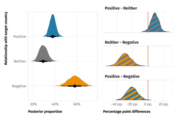
- Visualization for differences (Thread)
Significant Digits for Estimates
- Misc
- Notes from: Bayesian workflow book - Digits
- Before we can answer how many chains and iterations we need to run, we need to know how many significant digits we want to report
- MCMC in general doesn’t produce independent draws and the effect of dependency affects how many draws are needed to estimate different expectations
- Guidelines in general
- If the posterior would be close to a normal(μ,1), then
- For 2 significant digit accuracy,
- 2000 independent draws from the posterior would be sufficient for that 2nd digit to only sometimes vary.
- 4 chains with 1000 iterations after warmup is likely to give near two significant digit accuracy for the posterior mean. The accuracy for 5% and 95% quantiles would be between one and two significant digits.
- With 10,000 draws, the uncertainty is 1% of the posterior scale which would often be sufficient for two significant digit accuracy.
- For 1 significant digit accuracy, 100 independent draws would be often sufficient, but reliable convergence diagnostics may need more iterations than 100.
- For posterior quantiles, more draws may be needed (need more draws to get values towards the tails of the posterior)
- For 2 significant digit accuracy,
- Some quantities of interest may have posterior distribution with infinite variance, and then the ESS and MCSE are not defined for the expectation.
In such cases, use median instead of mean and median absolute deviation (MAD) instead of standard deviation.
Variance of parameter posteriors
as_draws_rvars(brms_fit) %>%
    summarise_draws(var = distributional::variance)
#>    variable  var
#>    <chr>    <dbl>
#>  1 mu        11.6
#>  2 tau      12.8
#>  3 theta[1]  39.7
#>  4 theta[2]  21.5
- If the posterior would be close to a normal(μ,1), then
- Steps
- Check convergence diagnostics for all parameters
- e.g. RHat, ESS, autocorrelation plots (see Diagnostics, Bayes)
- Look at the posterior for quantities of interest and decide how many significant digits is reasonable taking into account the posterior uncertainty (using SD, MAD, or tail quantiles)
- You want to be able to distinguish you upper or lower CI from the point estimate
- e.g. Point estimate is 2.1 and you upper CI is 2.1 then you want at least another significant digit.
- You want to be able to distinguish you upper or lower CI from the point estimate
- Check that MCSE is small enough for the desired accuracy of reporting the posterior summaries for the quantities of interest.
- Calculate the range of variation due to MC sampling for your paramter (See MCSE example)
- MC sampling error is the average amount of variation that’s expected from changing seeds and re-running the analysis
- If the accuracy is not sufficient (i.e. range is too wide), report less digits or run more iterations.
- Calculate the range of variation due to MC sampling for your paramter (See MCSE example)
- Check convergence diagnostics for all parameters
- Monte Carlo standard error (MCSE) - uncertainty about a parameter estimate due to MCMC sampling error
Packages
- {posterior} is the preferred package for brms objects
- {mcmcse} - methods to calculate MCMC standard errors for means and quantiles using sub-sampling methods. (Different calculation than used by Stan)
bayestestR::mcseuses Kruschke 2015 method of calculation
Example: brms, MCSE quantiles
# Coefficient and CI estimates for the "beta100" variable
as_draws_rvars(brms_fit) %>%
  subset_draws("beta100") %>%
  summarize_draws(mean, ~quantile(.x, probs = c(0.05, 0.95)))
#> variable  mean      5%   95%
#> beta100   1.966  0.673 3.242

as_draws_rvars(brms_fit) %>%
  subset_draws("beta100") %>% # select variable
  summarize_draws(mcse_mean, ~mcse_quantile(.x, probs = c(0.05, 0.95)))
#> variable  mcse_mean  mcse_q5 mcse_q95
#> beta100       0.013    0.036    0.033
- Specification
- “mcse_mean” and “mean” are available as preloaded functions that
summary_drawscan use out of the box - “mcse_quantile” (also in {posterior}) and “quantile” are not preloaded functions so they’re called as lambda functions
- “mcse_mean” and “mean” are available as preloaded functions that
- These are MCSE values for
- the summary estimate (aka point estimate) which is the mean of the posterior in this case
- And the CI values of that summary estimate
- Tail quantiles will have greater amounts of error sampling in the tails of the posterior than in the bulk (i.e. less accurate tail estimates)
- Fewer points, more uncertainty
- Calculate the range of variation due to Monte Carlo
- Multiply the MCSE values by 2, the likely range of variation due to Monte Carlo is ±0.02 for mean and ±0.07 for 5% and 95% quantiles
- Multiplying by 2, since I guess they’re assuming a normal distribution posterior, therefore estimate ± 1.96 * SE
- Multiply the MCSE values by 2, the likely range of variation due to Monte Carlo is ±0.02 for mean and ±0.07 for 5% and 95% quantiles
- Conclusion for “beta100” coefficient
- If the mean estimate for beta100 is reported as 2 (rounded up from 1.966), then there is unlikely to be any variation in that estimate due to MCMC sampling. (i.e. okay to report the estimate as 2)
- This is because
- 1.966 + 0.02 = 1.986 which would still be rounded up to 2
- 1.966 - 0.02 = 1.946 which would still be rounded up to 2
- This is because
- If the mean estimate for beta100 is reported as 2 (rounded up from 1.966), then there is unlikely to be any variation in that estimate due to MCMC sampling. (i.e. okay to report the estimate as 2)
- Draws and iterations
- With an MCSE in the 100ths (e.g. 0.07), 4 times more iterations would halve the MCSEs
- With an MCSE in the 1000ths (e.g. 0.007), 64 times more iterations would halve the MCSEs
- MCSEs depend on the quantity type. Continuous quantities (e.g. parameter estimates) have more information than discrete quantities (e.g. indicator values used to calculate probabilities).
- For example, above, the estimate for whether the temperature increase is larger than 4 degrees per century has high ESS, but the indicator variable contains less information (than continuous values) and thus much higher ESS would be needed for two significant digit accuracy.
Probabilistic Inference of Estimates
Misc
- Notes from: Bayesian workflow book - Digits
Example: probability that an estimate is positive
as_draws_rvars(brms_fit) %>%
  # binary 1/0, posterior samples > 0
  mutate_variables(beta0p = beta100 > 0) %>%
  subset_draws("beta0p") %>% # select variable
  summarize_draws("mean", mcse = mcse_mean)

#> variable  mean  mcse
#>   beta0p 0.993 0.001
99.3% probability the estimate is above zero +/- 0.2% (= 2*MCSE)
MCSE indicates that we have enough MCMC iterations for practically meaningful reporting that the probability that the variable (e.g. temperature) is increasing (i.e. slope is positive) is larger than 99%
Example: probability that an estimate > 1,2,3,4
as_draws_rvars(brms_fit) %>%
  subset_draws("beta100") %>%
  # binary 1/0 variable
  mutate_variables(beta1p = beta100 > 1,
                  beta2p = beta100 > 2,
                  beta3p = beta100 > 3,
                  beta4p = beta100 > 4) %>%
  subset_draws("beta[1-4]p", regex=TRUE) %>%
  summarize_draws("mean", mcse = mcse_mean, ESS = ess_mean)

#> variable  mean mcse  ESS
#>  beta1p 0.896 0.006 3020
#>  beta2p 0.487 0.008 4311
#>  beta3p 0.088 0.005 3188
#>  beta4p 0.006 0.001 3265
Taking into account MCSEs given the current posterior sample, we can summarise these as
- p(beta100>1) = 88%–91%,
- p(beta100>2) = 46%–51%,
- p(beta100>3) = 7%–10%,
- p(beta100>4) = 0.2%–1%.
To get these probabilities estimated with 2 digit accuracy would again require more iterations (16-300 times more iterations depending on the quantity), but the added iterations would not change the conclusion radically.perature in the center of the time range (instead defining prior for temperature at year 0).