Mixed Effects

Misc

Mixed Effects Model = Random Effects model = Multilevel model = Hierarchical model
- I’ve placed this model under econometrics, but it’s not considered an “econometrics” model given how widely it’s utilized across many disiplines and the history of its development.
Also see
Resources
- Bayesian Generalized Linear Mixed Effects Models for Deception Detection Analyses
  - Paper that’s an in-depth tutorial. Uses {brms}, {emmeans}, {parameters}
- Mixed Models in R by Michael Clark
Packages
- {lme4} - linear and generalized linear mixed-effects models; implemented using the ‘Eigen’ C++ library for numerical linear algebra and ‘RcppEigen’ “glue”.
  - Using {lmerTest} will produce a summary of lme4 models with pvals and dofs for coefficients
- {multilevelmod} - tidymodels wrapper for many mixed model packages.
  - {tidymodels} workflows (optional outputs: lmer, glmer, stan_glmer objects)
- {plm} - Linear models for panel data in an econometrics context; including within/fixed effects, random effects, between, first-difference, nested random effects. Also includes robust covariance estimators (e.g Newey-West), and model tests.
  - Formula syntax isn’t typical R format. The econometric estimators are unfamilar and will need extra research to figure out what they are, do, and how to use them appropriately.
- {glmmTMB} - for fitting generalized linear mixed models (GLMMs) and extensions
  - Wide range of statistical distributions (Gaussian, Poisson, binomial, negative binomial, Beta …) and zero-inflation.
  - Fixed and random effects models can be specified for the conditional and zero-inflated components of the model, as well as fixed effects for the dispersion parameter.
- {spaMM} - Inference based on models with or without spatially-correlated random effects, multivariate responses, or non-Gaussian random effects (e.g., Beta).
- {merTools} - Allows construction of prediction intervals efficiently from large scale linear and generalized linear mixed-effects models
  - Also has tools for analyzing multiply imputed mixed efffects models
  - Comes with a shiny app to explore the model
Advantages of a mixed model ($y \sim x + (x \;|\; g)$) vs a linear model with an interaction ($y \sim x \ast g$)
- From T.J. Mahr tweet
- Conceptual: Assumes participant means are drawn from the same latent population
- Computational: partial pooling / smoothing
- Both will have very similar parameter estimates when the data is balanced with few to no outliers
  - Linear least squares regression can overstate precision, producing t-statistics for each fixed effect that tend to be larger than they should be; the number of significant results in LLSR are then too great and not reflective of the true structure of the data
  - Standard errors are underestimated in the interaction model.
    - Doesn’t account for dependence in the repeated measure for each subject
  - For unbalanced data w/some group categories having few data points or with outliers, the mixed effects model regularizes/shrinks/smooths the estimates to the overall group (i.e. population) mean
- Example of model formula interpretation
Mixed Effects and Longitudinal Data
- Harrell (article)
  - Says that Mixed Models models can capture within-subject correlation of repeated measures over very short time intervals but not over extended time intervals where autocorrelation comes into play
    - Example of a short interval is a series of tests on a subject over minutes when the subject does not fatigue
    - Example of a long interval is a typical longitudinal clinical trial where patient responses are assessed weekly or monthly
  - He recommends a Markov model for longitudinal RCT data (see bkmks)
- Bartlett
  - Mixed model repeated measures (MMRM) in Stata, SAS and R
    - Tutorial; uses {nlme::gls}

Considerations

Motivation for using a Random Effects model
- You think the little subgroups are part of some bigger group with a common mean effect
  - e.g. Multiple observations of a single person, or multiple people in a school, or multiple schools in a district, or multiple varieties of a single kind of fruit, or multiple kinds of vegetable from the same harvest, or multiple harvests of the same kind of vegetable, etc.
- These subgroup means significantly deviate from the big group mean.
  - i.e. We suspect there to be between-subject variance and not just within-subject variance (linear model).
    
    Within-Subject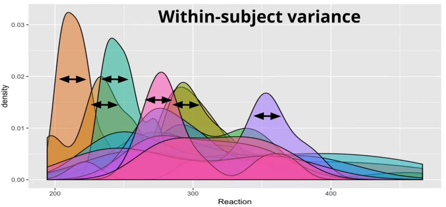
    
    Between-Subject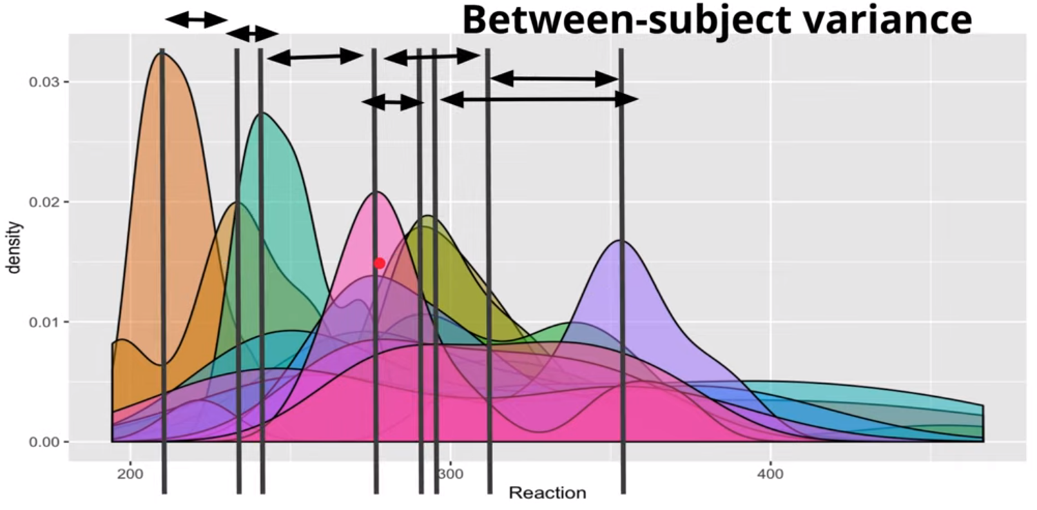
    - The Between-Subject Variance isn’t clearly depicted IMO. The Between-Subject Variance captures the differences between individual subjects or groups in their average responses or outcomes. It can be understood better by looking at the sample formula where the grand mean is subtracted from each subject’s mean.
      
      \[ \text{Between-Subject Variance} = \frac{\sum_{i=1}^{k} n_i (\bar{X}_i - \bar{X})^2}{k-1} \]
      - $k$ is the number of groups or levels of the independent variable.
        
        Denominator is a dof term.
      - $n_i$ is the number of observations in the i^th group.
      - $\bar X_i$ is the mean of the observations in the i^th group.
      - $\bar X$ is the grand mean.
- These deviations follow a distribution, typically Gaussian.
  - That’s where the “random” in random effects comes in: we’re assuming the deviations of subgroups from a parent follow the distribution of a random (Gaussian) variable
    - The variation between subgroups is assumed to have a normal distribution with a 0 mean and constant variance (variance estimated by the model).
  - GEEs are a semi-parametric option for panel data (See Regression, Other >> Generalized Estimating Equations (GEE))
Fixed Effects or Random Effects?
- If there’s likely correlation between unobserved group/cases variables (e.g. individual talent) and treatment variable (i.e. E(α|x) != 0) AND there’s substantial variance between group units, then FE is a better choice (See Econometrics, Fixed Effects >> One-Way Fixed Effects >> Assumptions)
- If cases units change little, or not at all, across time, a fixed effects model may not work very well or even at all (SEs for a FE model will be large)
  - The FE model is for analyzing within-units variance
- Do we wish to estimate the effects of variables whose values do not change across time, or do we merely wish to control for them?
  - FE: these effects aren’t estimated but adjusted for by explicitly including a separate intercept term for each individual (αi) in the regression equation
  - RE: estimates these effects (might be biased if RE assumptions violated)
    - The RE model is for analyzing between-units variance
- The amount of within-unit variation relative to between-unit variation has important implications for these two approaches
  - Article with simulated data showed that within variation around sd < 0.5 didn’t detect the effect of explanatory variable but ymmv (depends on # of units, observations per unit, N)
- Durbin–Wu–Hausman test ({plm::phtest})
  - If H0 is not rejected, then both FE and RE are consistent but only RE is efficient. $\rightarrow$ use RE but if you have a lot of data, then FE is also fine.
  - If H0 is rejected, then only FE is consistent $\rightarrow$ use FE
- ICC > 0.1 is generally accepted as the minimal threshold for justifying the use of Mixed Effects Model (See Diagnostics >> ICC)
Pooling
- Complete pooling - Each unit is assumed to have the same effect
  - Example: County is the grouping variable and radon level is the outcome
    - All counties are alike.
      - i.e. all characteristics of counties that affect radon levels in houses have the statistically same effect across counties. Therefore, the variable has no information.
    - Run a single regression to estimate the average radon level in the whole state.
      - lm(radon_level ~ predictors)
      - Note that “county” is NOT a predictor in this model
- No pooling - All units are assumed to have independent effects
  - Example: County is the grouping variable (although not a predictor in this case) and radon level is the outcome
    - All counties are different from each other.
      - i.e. there are no common characteristics of counties that affect radon levels in houses. Any characteristic a county has that affects radon levels is unique to that county.
    - Run a regression for each county to estimate the average radon level for each county.
      - lm(radon_level ~ 0 + county + predictors
      - Using the “0 +” formula removes the common intercept which means each county will get it’s own intercept
- Partial pooling - Each unit is assumed to have a different effect, but the data for all of the observed units informs the estimates for each unit
  - Example: County is the grouping variable (random effect) and radon level is the outcome
    - All counties are similar each other.
      - i.e. all charcteristics of counties that affect radon levels in house have statistically varying effects sizes depending on the particular county
    - Run a multi-level regression to share information across counties.
      - lmer(radon_level ~ predictors + (1 + predictor | county))
  - This can be a nice compromise between estimating an effect by completely pooling all groups, which masks group-level variation, and estimating an effect for all groups completely separately, which could give poor estimates for low-sample groups.
  - If you have few data points in a group, the group’s effect estimate will be based partially on the more abundant data from other groups. (2 min video)
    - This is called Regularization. Subjects with fewer data points will have their estimates pulled to the grand mean more than subjects with more data points.
      - The grand mean will be the (Intercept) value in the Fixed Effects section of the summary.
    - You can visualize the amount of regularization by comparing the conditional modes (see Model Equation >> Conditional Modes) to the group means in the observed data.
      - Example (link)
        
        Code
        
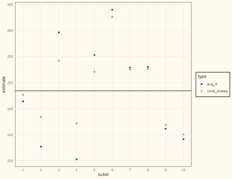
        rt_lme_mod <- lmer(rt ~ 1 + (1|subid), dat) comparison_dat <- dat |> summarize(avg_rt = mean(rt), .by = subid) |> mutate(cond_modes = coef(rt_lme_mod)$subid[[1]]) |> tidyr::pivot_longer( cols = c(avg_rt, cond_modes), names_to = "type", values_to = "estimate" ) ggplot(comparison_dat, aes(x = subid, y = estimate, color = type)) + geom_point() + scale_color_manual(values = c("#195198", "#BD9865")) + geom_hline(yintercept = lme4::fixef(rt_lme_mod)[[1]]) + # overall intercept/grand mean scale_x_continuous(breaks = seq(0 , 10, 1), minor_breaks=seq(0, 10,1)) + theme_notebook()
        
        The conditional modes (gold) are all closer to the horizontal line which represents the grand mean.
        
        There are few data points for each of the first five subjects, so in general, they are pulled more than the last five subjects which have many more data points.
        
        i.e. The differences between the observed means (blue) and conditional modes (gold) are greater in the first five subjects than the last five subjects
        
        Points already close to the grand mean can’t be pulled as much since they’re already very close to the grand mean (e.g. subject 1)
  - Partial pooling is typically accomplished through hierarchical models. Hierarchical models directly model the population of units. From a population model perspective, no pooling corresponds to infinite population variance, whereas complete pooling corresponds to zero population variance.
Variable Assignment
- Questions (article has examples)
  - Can the groups we see be considered the full population of possible groups we could see, or are they more like a random sample of a larger set of groups?
    - Full Population: Fixed
    - Random Sample: Random
  - Do we want to estimate a coefficient for this grouping, or do we just want to account for the anticipated structure that the groups may impose on our observations?
    - Y: Fixed
    - N: Random
- Fixed Effects provide estimates of mean-differences or slopes.
  - “Fixed” because they are effects that are constant for each subject/unit
  - Should include within-subject variables (e.g. random effect slope variables) and between-subject variables (e.g. gender)
  - Level One: variables measured at the most frequently occurring observational unit
    - i.e. Vary for each repeated measure of a subject and vary between subjects
      - In the dataset, these variables that (for the most part) have different values for each row
      - Time-dependent if you have longitudinal data
    - For a RE model, these are usually the adjustment variables
      - e.g. Conditioning on a confounder
  - Level Two: variables measured at the observational unit level
    - i.e. Constant for each repeated measure of a subject but vary between each subject
    - For a RE model, these are usually the treatment variables or variables of interest
      - They should contain the information about the between-subject variation
    - If a factor variable, it has levels which would not change in replications of the study
- Random Effects estimate of variation between and within subgroups
  - Intercepts variables (e.g. v1 in Specification and Notation) should be grouping variables (i.e. discrete or categorical) (e.g school, department)
  - Slopes variables (e.g. v2 in Specification and Notation) should be continuous within-subject variables (e.g time)
    - These variables should also be included in the fixed effects
  - Quantifies how much of the overall variation can be attributed to that particular variable.
    - Example: the variation in beetle DAMAGE was attributable to the FARM at which the damage took place, so you’d cluster by FARM (1|FARM)
  - If you want slopes to vary according to a variable, the variation of slopes between-units will be a random effect
    - Usually a level 2 fixed effect variable
  - If you want intercepts to vary according to a variable, the variation of intercepts between-units will be a random effect
    - This will the unit/subject variable (e.g student id, store id) that has the repeated observations
  - Typically categorical variables that we are not interested in measuring their effects on the outcome variable, but we do want to adjust for. This variation might capture effects of latent variables.
    - This factor variable has levels which can be thought of as a sample from a larger population of factor levels (e.g. hockey players)
    - Example: 2 hockey players both averaged around 20 minutes per game last year (fixed variable). Predictions of the amount of points scored by just accounting for this fixed variable would produce similar results. But using PLAYER as a random variable will capture the impact of persistent characteristics that might not be observable elsewhere in the explanatory data. PLAYER can be thought of as a proxy for “offensive talent” in a way.
  - If the values of the variable were chosen at random, then you should cluster by that variable (i.e. choose as the random variable)
    - Example: If you can rerun the study using different specific farms (i.e .different values of the FARM factor, see above) and still be able to draw the same conclusions, then FARM should be a random effect.
      - However, if you had wanted to compare or control for these particular farms, then Farm would be “fixed.”
      - Say that there is nothing about comparing these specific fields that is of interest to the researcher. Rather, the researcher wants to generalize the results of this experiment to all fields. Then, FIELD would be “random.”
  - If the random effects are correlated with variables of interest (fixed effects), leaving them out could lead to biased fixed effects. Including them can help more reliably isolate the influence of the fixed effects of interest and more accurately model a clustered system.
  - To see individual random effects: lme4::ranef(lme_mod) or lme4::ranef(tidy_mod$fit)

Model Equation

Misc
- Notes from Video Playlist: Mixed Model Series
  - Companion resource to the videos. Contains more details, code, and references.
- Also see the BMLR Chapter 8 section for a similar description
- It’s useful to consider the model in two stages even though all the parameters are estimated at the same time (See Combined equation)
  - If all subjects have the same number of observations, the 2-Stage approach and Mixed Model should have very similar results.
  - A use case for the 2-Stage approach is comparing the correlation between a dependent variable and two independent variables (i.e. $Y \sim X_1$ and $Y \sim X_2$) when the data is repeated measures.
    - Subjects (aka units) should be balanced if you want valid standard errors (See Issues)
    - Execute the 2-Stage approach for both model formulas and the 2nd Stage’s coefficient will be the Pearson Correlation coefficient. (Code from MMS Resource, also mentioned at the end of video 4 or 5)
- Issues with only using a 2-stage approach
  - Not all random effects structures can be modelling using 2 stages
  - The variance estimate in the 2^nd stage will be incorrect
    - The standard errors will be too small which will inflate the type I error rate.
    - This is most prevalent is designs with an imbalanced binary group variable fixed effect (e.g. treatment/control) where one group has fewer subjects than the other group (See MMS resource/video 6)
    - There is a loss of power in designs that have an imbalance in the binary group variable and imbalance in the number of observations per subject. (See MMS resource/video 6)
  - Mixed Effects models have built-in regularization.
2-Stage Model
- 1^st Stage
  \[ Y_i = \beta_iZ_i + \epsilon_i, \quad \epsilon \sim \mathcal N (0, \sigma^2I_{n_i}) \]
  - $\beta_i Z_i$ is the slope and intercept times the design matrix for subject $i$
  - $\epsilon$ is the within-subject error
  - $\sigma^2I_{n_i}$ is the within-subject variance matrix which is just a diagonal matrix with $\sigma^2$s along the diagonal which is the within-subject variation.
    - In this case $\sigma^2$ is constant for all subjects. (i.e. the variance is pooled). Preferred method when you have small data which makes estimation of subject-level variance difficult.
    - The remaining unexplained variance at the subject-level after accounting for the between-subject variance.
  - $\beta_i$ says that there’s a slope for each subject which makes sense if there’s repeated measures
- 2^nd Stage
  \[ \beta_i = \beta A_i + b_i, \quad b_i \sim \mathcal N (0, G) \]
  - $\beta$ is a group parameter estimate (i.e. avarage intercept and average slope across all subjects). The intercept will be the grand mean and other coefficients are the fixed effects coefficients.
  - $A_i$ is a design matrix
    - Typically an identity matrix unless it’s a more complex model
  - $b_i$ is the random effect between-subject error. Isn’t actually a subject-level vector of residuals. It’s an estimated distribution — typically Gaussian.
    - $G$ is a 2 $\times$ 2 Covariance matrix (in this case). Same for all subjects.
      - Upper-Left: Between-Subject Intercept Variance
      - Bottom-Right: Between-Subject Slope Variance
      - Upper-Right: Covariance between slope and intercept (i.e. a dependence between slope and intercept)
        
        Same for Bottom-Left.
- Combined: $Y_i = \beta Z_i A_i + b_i Z_i + \epsilon_i$

Term Estimates

library(lme4); library(Matrix)
data("sleepstudy")
# varying slopes and varying intercepts
lmer_mod <- 
  lmer(Reaction ~ 1 + Days + (1 + Days | Subject),
       sleepstudy,
       REML = 0)
summary(lmer_mod)

#> Random effects:
#>  Groups   Name        Variance Std.Dev. Corr
#>  Subject  (Intercept) 565.48   23.780       
#>           Days         32.68    5.717   0.08
#>  Residual             654.95   25.592       
#> Number of obs: 180, groups:  Subject, 18

$\sigma^2$ is Residual = 654.95 (variance of the within-subject error)
- Interpreted as the within-subject variance. It’s the average variance of each subject’s response value in relation to their within-subject average response value.
$G$
- Subject (Intercept) = 565.52 (Variance) (Upper-Left: Between-Subject Intercept Variance)
- Days = 32.48 (Variance) (Between-Subject Slope Variance)
- Days = 0.08 (Corr) (Upper-Right: Covariance between slope and intercept)

Conditional Modes
- Currently I’m not sure what these are. I’ve read/watched a few different things that state or imply different definitions of the term.
  - Fitted Values: These are essentially just fitted values for a mixed effects model. The difference is having a different intercept value for each subject id and/or a different slope for each subject id. (Mumford from Mixed Models Series)
    - Mumford is following a book on Longitudinal data. I’m leaning towards this definition.
  - Random Slopes/Intercepts: These take each subject’s random effect and adds it the fixed effect (model avereage) (Michael Clark implies this in Mixed Models in R)
  - Random Effects: {lme4}’s functional documentation and vignette imply that these are conditional modes through their function defintions (Bates et al)
- AKA BLUPs (Best Linear Unbiased Predictor). I’ve seen this terminology discouraged a couple different places though.
  - I think BLUPs comes from the original paper and Conditional Modes comes from the author of {lme4}. Both should be lost to history.
- Conditional Modes ($\hat \beta$) as function of OLS and the Mixed Model Grand Mean (aka fixed effects intercept)
  
  \[ \begin{align} &\hat\beta_i = W_i\hat\beta_i^{OLS}+(I_q-W_i)A_i\hat\beta \\ &\text{where} \quad W_i= \frac{G}{G+\sigma^2(Z_i'Z_i)^{-1}} \end{align} \]
  - Not essential to know this but it gives you insight to how the 2-Stage model and the Mixed Model estimates will differ. It also gives insight into what affects the amount of Regularization. (See Considerations >> Partial Pooling)
  - The top equation shows that if the weight $W$ is large (e.g. $1$), then the OLS estimate (subject-level means) will be close the mixed effects estimate
  - The bottom equation shows that if the Between-Subject Variance ($G$) is much larger than the Within-Subjects Variance ($\sigma^2$), then the weight will be large (i.e. close to $1$).
  - For a simple varying intercepts model $Z'Z$ is just $\frac{1}{N_i}$. For a small, $N_i$, $W$ will be small which leads to the grand mean estimate, $\hat\beta$, dominating the conditional mode equation which means more regularization for that subject.
- Get the conditional modes whatever they might be:
  - Fitted Values:
```
fitted(lme_mod)
# or
predict(lme_mod,
        new_data)
```
  - Random Slopes or Intercepts:
```
rand_int <- ranef(lme_mod)$group_var$`(Intercept)` + fixef(lme_mod$group_var$`(Intercept)`)
rand_slope <- ranef(lme_mod)$group_var$slope_var + fixef(lme_mod$group_var$slope_var)
```
    - If conditonal modes are just the random effects then ranef(lme_mod)
- Examples: Manual Method (Assumes Fitted Values are Conditional Modes)
  - Fixed Effect + Varying Intercepts
  - Varying Slopes and Intercepts
  glimpse(dat.mod) #> Rows: 1,500 #> Columns: 3 #> $ id <fct> 1, 1, 1, 1, 1, 1, 1, 1, 1, 1, 1, 1, 1, 1, 1, 1, 1, 1, 1, 1, 1, 1, 1, 1, 1, 1, 1, 1, 1, 1, 2, 2, 2, 2, 2… #> $ y <dbl> -18.5954522, -0.3249434, 12.8352423, -6.1749271, 7.1217294, 14.5693488, -2.4363220, -23.1468863, -4.016… #> $ grp.all <dbl> 1, 1, 1, 1, 1, 1, 1, 1, 1, 1, 1, 1, 1, 1, 1, 1, 1, 1, 1, 1, 1, 1, 1, 1, 1, 1, 1, 1, 1, 1, 1, 1, 1, 1, 1… mod.lmer <- lmer(y ~ grp.all + (1 | id), dat.mod) # Using the model equation group.vec <- rep(c(1, 0), each = 25) # distinct group.all values/num of subjects cond.modes <- coef(mod.lmer)$id[, 1] + coef(mod.lmer)$id[, 2]*group.vec # Using predict() new_dat <- dat.mod |> distinct(id, grp.all) me_preds <- predict(mod.lmer2, new_dat) head(cond.modes); head(as.numeric(me_preds)) #> [1] 10.425813 14.724778 12.815295 8.282038 4.234039 9.870040 #> [1] 10.425813 14.724778 12.815295 8.282038 4.234039 9.870040
  
  In a basic RCT design, grp.all would be your treatment/control variable and id would be your subject (aka unit) id.
  fm1 <- lmer(Reaction ~ Days + (Days|Subject), sleepstudy) # random effects re_intercepts <- ranef(fm1)$Subject$`(Intercept)` re_slopes <- ranef(fm1)$Subject$`Days` # fixed effects fe_intercept <- fixef(fm1)[1] # grand mean fe_slope <- fixef(fm1)[2] # average slope for Days random_intercepts <- fe_intercept + re_intercepts random_slopes <- fe_slope + re_slopes random_df <- tibble( Subject = as.factor(levels(sleepstudy$Subject)), random_slopes = random_slopes, random_intercepts = random_intercepts ) # Join each random_* to the repeated measures rows for Subject random_df_full <- sleepstudy |> select(Subject) |> left_join(random_df, by = "Subject") cond_modes <- random_df_full$random_intercepts + (random_df_full$random_slopes * sleepstudy$Days) fitted_values <- fitted(fm1) head(cond_modes); head(as.numeric(fitted_values)) #> [1] 253.6637 273.3299 292.9962 312.6624 332.3287 351.9950 #> [1] 253.6637 273.3299 292.9962 312.6624 332.3287 351.9950
  
  Shows how random effects are used to get the conditional modes.
  \[ \begin{aligned} \text{Conditional Modes}_i &= (\text{Random Effect}_{\text{intercept}_i} + \text{Fixed Effect}_{\text{intercept}}) \\ &+ (\text{Random Effect}_{\text{Days}_i} + \text{Fixed Effect}_{\text{Days}}) \times \text{Days}_{i,j} \end{aligned} \]
  
  Days is the repeated measures id so to speak. In this study, each Subject ($i$) has 10 Days ($j$) of follow-up measurements

Assumptions

No Time-Constant Unobserved Heterogeneity: $\mathbb{E}(\alpha_i\;|\;x_{it}) = 0$
- i.e. No correlation between time-invariant valued, unobserved variables (aka random effect variable) and the explanatory variable of interest (e.g. treatment)
  - Time-Invariant Valued, Unobserved Variables: Variables that are constant across time for each unit and explain variation between-units
    - e.g. If random effect variable (aka clustering variable) is the individual, then the “time-invariant, unobserved” variable could be something latent like talent or something measureable like intelligence or socio-economic status. Whatever is likely to explain the variance between-units in relation to the response.
- The effect that these variables have must also be time-invariant
  - e.g. The effect of gender on the outcome at time 1 is the same as the effect of gender at time 5
  - If effects are time-varying, then an interaction of gender with time could be included
- It’s not reasonable for this to be exactly zero in order to use a mixed effected model, but for situations where there’s high correlation, this model should be avoided
- Example: Violation
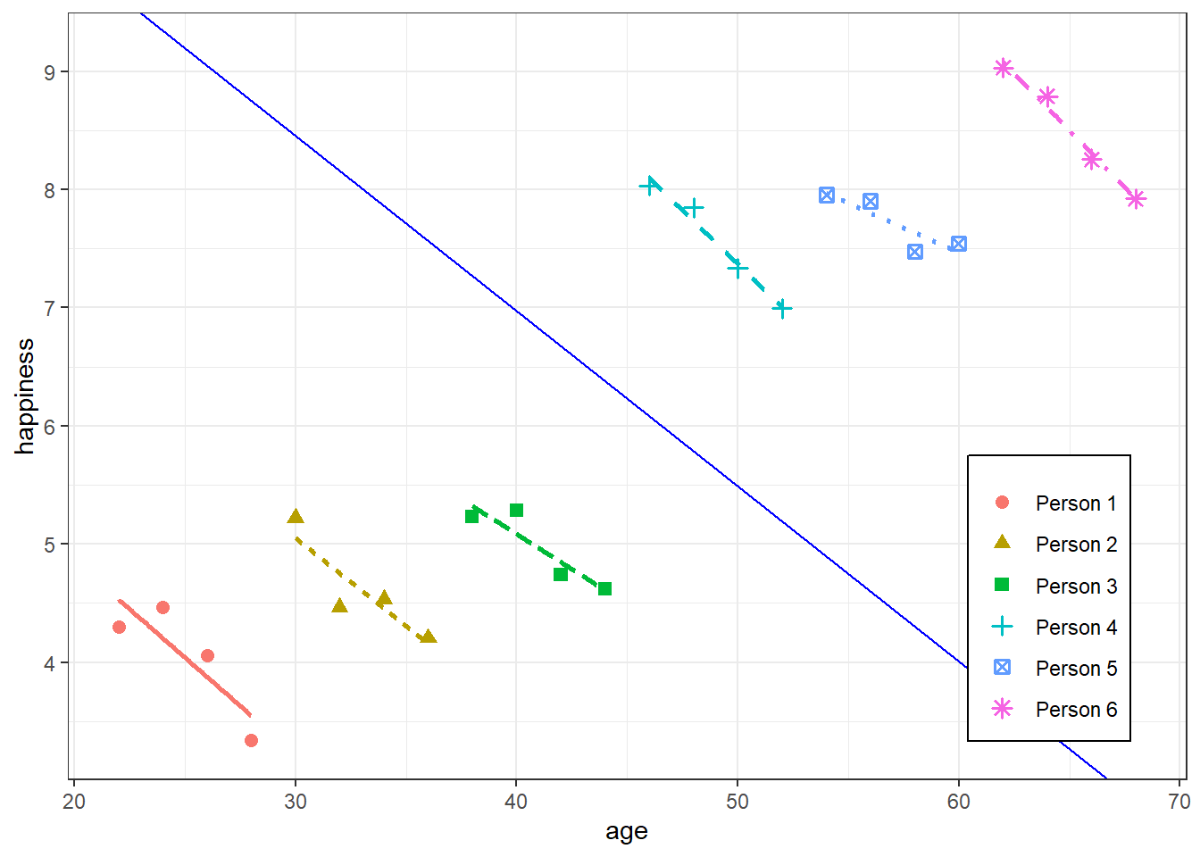
  - Each group’s x values get larger from left to right as each group’s α (aka y-intercepts) for each unit get larger
    - i.e. Mixed-Effects models fail in cases where there’s very high correlation between group intercepts and x, together with large between-group variability compared to the within-group variability
  - **FE model would be better in this case
    - Gelman has a paper that describes how a mixed effect model can be fit in this situation though
No Time-Varying Unobserved Heterogeneity: $\mathbb{E}(\epsilon_{it}|x_{it}) = 0$
- i.e No endogeneity (no correlation between the residuals and explanatory variable of interest)
- If violated, there needs to be explicit measurements of omitted time-invariant variables (see 1st assumption for definition) if they are thought to interact with other variables in the model.

Specifications and Notation

Every variable within the parentheses is for the random effects. Variables outside the parentheses are fixed effects.
Varying Intercepts: (1 | v1)
- AKA Random Intercepts, where each level of the random variable (our random effect) had an adjustment to the overall intercept
- Example: Each department (random variable) has a different starting (intercepts) salary (outcome variable) for their faculty members (observations), while the annual rate (slope) at which salaries increase is consistent across the university (i.e. effect is constant between-departments)
  
  \[ \widehat{\text{salary}}_i = \beta_{0 j[i]} + \beta_1 \cdot \text{experience}_i \]
  - Where j[i] is the index for department
  - This strategy allows us to capture variation in the starting salary (intercepts) of our faculty
Varying Slopes: (0 + v2| v1)
- AKA Random Slopes, which would allow the effect of the v2 to vary by v1
  - i.e. v2 is a predictor whose effect varies according to the level of the grouping variable, v1.
- i.e. A slope for each level of the random effects variable
- Example: faculty salary (outcome) increase at different rates (slopes) depending on the department (random variable).
  
  \[ \widehat{\text{salary}}_i = \beta_0 + \beta_{1 j[i]} \cdot \text{experience}_i \]
  - Where j[i] is the index for department
  - This strategy allows us to capture variation in the change (slopes) in salary
Varying Slopes and Intercepts: (1 + v2 | v1) or just (v2 | v1) (See examples)
- See above for descriptions of each
- Example: Each department (random variable) has a different starting (intercepts) salary (outcome variable) for their faculty members (observations), while the annual rate (slope) at which salaries increase varies depending on department
  
  \[ \widehat{\text{salary}}_i = \beta_{0 j[i]} + \beta_{1 j[i]} \cdot \text{experience}_i \]
  - Where j[i] is the index for department
  - See above for descriptions of each type of variation this strategy captures
Nested Effects
- e.g. Studying test scores (outcome variable) within schools (random variable) that are within districts (random variable)
- *For {lme4}, using Nested or Crossed notation is NOT important for parameter estimation. Both specifications will produce exactly the same results.*
  - See link for more details and references
  - The interpretation of the results are also the same
  - The only situation where it does matter is if the nested variable (e.g. v2) does not have unique values.
    - For example, if wards are nested within hospitals and there’s a ward named 11 that’s in more than one hospital except that they’re obviously different wards.
    - In that situation, you can either create a unique ward id or use the nested notation.
- Notation: (1 | v1 / v2) or (1 | v1) + (1 | v1:v2)
  - Says intercepts varying among v1 and v2 within v1.
  - e.g. schools is v2 and districts is v1
- Unit IDs may be repeated within groups.
  - Example: lme4::lmer(score ~ time + (time | school/student_id))
    - The random effect at this level is the combination of school and student_id, which is unique.
    - You can verify this by calling ranef on the fitted model. It’ll show you the unique combinations of student_ids within schools used in the model.
Crossed Effects
- Use when you have more than one grouping variable, but those grouping variables aren’t nested within each other.
- *For {lme4}, using Nested or Crossed notation is NOT important for parameter estimation. Both specifications will produce exactly the same results.*
  - See link for more details and references
  - The interpretation of the results are also the same
  - The only situation where it does matter is if the nested variable (e.g. v2) does not have unique values.
    - For example, if wards are nested within hospitals and there’s a ward named 11 that’s in more than one hospital except that they’re obviously different wards.
    - In that situation, you can either create a unique ward id or use the nested notation.
- Such models are common in item response theory, where subject and item factors are fully crossed
  - Two variables are said to be “fully crossed” when every combination of their levels appears in the data.
  - When variables are fully crossed, it means that their effects on the response variable can be estimated independently and without any confounding or aliasing. This allows you to properly disentangle and interpret the main effects and potential interactions between the variables.
- Notation: (1 | v1) + (1 | v2) says there’s an intercept for each level of each grouping variable.
Uncorrelated Random Effects
- If you have model where slopes and intercepts aren’t very correlated and would like to reduce the complexity (i.e. fewer dofs), then specifying an uncorrelated model means fewer parameters have to be estimated which lowers your degrees of freeedom.
  - This can also be a potential solution to nonconvergence issues.
- Notation: (x || g) or (1 | g) + (0 + x | g)
- Ideally these models should be restricted to cases where the predictor is measured on a ratio scale (i.e., the zero point on the scale is meaningful, not just a location defined by convenience or convention).
  - This is from a {lme4} vignette. They used a Day variable that was used as a varying slope variable as an example that meets the condition since Day = 0 is meaningful (even though it’s not a ratio I guess).

Strategy

Misc
- Also see
  - BMLR Ch 8 >> Model Building Workflow: Simple to Complex
  - Model Building, Concepts >> Misc
- Begins with a saturated fixed effects model, determines variance components based on that, and then simplifies the fixed part of the model after fixing the random part.
Overall:
- EDA
- Fit some simple, preliminary models, in part to establish a baseline for evaluating larger models.
- Then, build toward a final model for description and inference by attempting to add important covariates, centering certain variables, and checking model assumptions.
Process
- EDA at each level (See EDA, Multilevel, Longitudinal)
- Examine models with no predictors to assess variability at each level
- Create Level One models: starting simple and adding terms as necessary (See Considerations >> Variable Assignment >> Fixed Effects )
- Create Level Two models: starting simple and adding terms as necessary (See Considerations >> Variable Assignment >> Fixed Effects)
  - Beginning with the equation for the intercept term.
- Examine the random effects and variance components (See Considerations >> Variable Assignment >> Random Effects)
  - Beginning with a full set of error terms and then removing covariance terms and variance terms where advisable
    - e.g. When parameter estimates are failing to converge or producing impossible or unlikely values
  - See Specifications and Notation for different RE modeling strategies.

Examples

Example: {lme4}
- From Estimating multilevel models for change in R
- usl is UK sociological survey data
  - logincome is a logged income variable
  - pidp is the person’s id
  - wave0 is the time variable that’s indexed at 0
library(lme4) # unconditional means model (a.k.a. random effects model) m0 <- lmer(data = usl, logincome ~ 1 + (1 | pidp)) # check results summary(m0) ## Linear mixed model fit by REML ['lmerMod'] ## Formula: logincome ~ 1 + (1 | pidp) ## Data: usl ## ## REML criterion at convergence: 101669.8 ## ## Scaled residuals: ## Min 1Q Median 3Q Max ## -7.2616 -0.2546 0.0627 0.3681 5.8845 ## ## Random effects: ## Groups Name Variance Std.Dev. ## pidp (Intercept) 0.5203 0.7213 ## Residual 0.2655 0.5152 ## Number of obs: 52512, groups: pidp, 8752 ## ## Fixed effects: ## Estimate Std. Error t value ## (Intercept) 7.162798 0.008031 891.8
- Interpretation
  
  Fixed effects:
  
  (Intercept) = 7.162798, which is the grand mean
  
  Says that the average of the individual averages of log income is 7.162798
  
  Random effects:
  
  Everything that varies by pidp
  
  Between-case (or person, group, cluster, etc.) variance: (Intercept) = 0.5203
  
  Within-case (or person, group, cluster, etc.) variance: Residual = 0.2655
- ICC
  
  $\frac{0.520}{0.520 + 0.265} = 0.662$
  
  Says about 66% of the variation in log income comes between people while the remaining (~ 34%) is within people.
library(lme4) # unconditional change model (a.k.a. MLMC) m1 <- lmer(data = usl, logincome ~ 1 + wave0 + (1 | pidp)) summary(m1) ## Linear mixed model fit by REML ['lmerMod'] ## Formula: logincome ~ 1 + wave0 + (1 | pidp) ## Data: usl ## ## REML criterion at convergence: 100654.8 ## ## Scaled residuals: ## Min 1Q Median 3Q Max ## -7.1469 -0.2463 0.0556 0.3602 5.7533 ## ## Random effects: ## Groups Name Variance Std.Dev. ## pidp (Intercept) 0.5213 0.7220 ## Residual 0.2593 0.5092 ## Number of obs: 52512, groups: pidp, 8752 ## ## Fixed effects: ## Estimate Std. Error t value ## (Intercept) 7.057963 0.008665 814.51 ## wave0 0.041934 0.001301 32.23 ## ## Correlation of Fixed Effects: ## (Intr) ## wave0 -0.375
- Model
  
  1 covariate
  
  Random Effect: Cases; Fixed Effect: Time
- Interpretation
  
  Fixed effects:
  
  (Intercept) = 7.057; the expected log income at the beginning of the study (wave 0).
  
  wave0 = 0.0419
  
  The average rate of change with the passing of a wave.
  
  I don’t think this is a percentage. It’s the same as a standard OLS regression interpretation.
  
  So after each wave, individual log income is expected to slowly increase by 0.041 on average.
  
  Random Effects
  
  Everything varies by pidp
  
  Between-Case (or person, group, cluster, etc.) variance in log income: (Intercept) = 0.5213
  
  Within-Case (or person, group, cluster, etc.) variance in log income: Residual = 0.2593
  
  So this stuff is still very similar numbers as the varying intercept-only model
- Visualize Effect
  
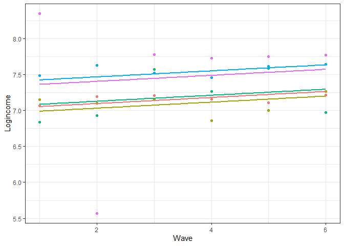
  Code
  
  usl$pred_m1 <- predict(m1) usl %>% filter(pidp %in% 1:5) %>% # select just five individuals ggplot(aes(wave, pred_m1, color = pidp)) + geom_point(aes(wave, logincome)) + # points for observed log income geom_smooth(method = lm, se = FALSE) + # linear line showing wave0 slope theme_bw() + labs(x = "Wave", y = "Logincome") + theme(legend.position = "none")
  
  wave was indexed to 0 for the model but now wave starts at 1. He might’ve reverted wave to have a starting value of 1 for graphing purposes
  
  Lines show the small, positive, fixed effect slope for wave0
  
  Parallel lines means we assume the change in log income over time is the same for all the individuals
  
  i.e. We assume there is no between-case variation in the rate of change.
library(lme4) # unconditional change model (a.k.a. MLMC) with re for change m2 <- lmer(data = usl, logincome ~ 1 + wave0 + (1 + wave0 | pidp)) summary(m2) ## Linear mixed model fit by REML ['lmerMod'] ## Formula: logincome ~ 1 + wave0 + (1 + wave0 | pidp) ## Data: usl ## ## REML criterion at convergence: 98116.1 ## ## Scaled residuals: ## Min 1Q Median 3Q Max ## -7.8825 -0.2306 0.0464 0.3206 5.8611 ## ## Random effects: ## Groups Name Variance Std.Dev. Corr ## pidp (Intercept) 0.69590 0.8342 ## wave0 0.01394 0.1181 -0.51 ## Residual 0.21052 0.4588 ## Number of obs: 52512, groups: pidp, 8752 ## ## Fixed effects: ## Estimate Std. Error t value ## (Intercept) 7.057963 0.009598 735.39 ## wave0 0.041934 0.001723 24.34 ## ## Correlation of Fixed Effects: ## (Intr) ## wave0 -0.558
- Model
  
  Random Effect: outcome (i.e. intercept) by cases
  
  Time Effect by cases
  
  Fixed Effect: time
  
  (1 + wave0 | pidp) - Says let both the intercept (“1”) and wave0 vary by pidp - Which means that average log income varies by person and the rate of change (slope) in log income over time (wave0 fixed effect) varies by person.
- Interpretation
  
  Out of all the models this one has the lowest REML
  
  Fixed effects:
  
  (Intercept) = 7.057963: The expected log income at the beginning of the study (wave 0).
  
  wave0 = 0.0419
  
  The average rate of change with the passing of a wave.
  
  I don’t think this is a percentage. It’s the same as a standard OLS regression interpretation.
  
  So after each wave, individual log income is expected to slowly increase by 0.041 on average.
  
  Random effects:
  
  Everything that varies by pidp
  
  Within-Case (or person, group, cluster, etc.) variance of log income:
  
  Residual = 0.21052
  
  How much each person’s log income varies in relation to her average log income
  
  Between-Case (or person, group, cluster, etc.) variance of log income:
  
  (Intercept) = 0.69590
  
  How much each person’s average log income varies in relation to the group’s average log income (The fixed effect intercept which is also the grand mean)
  
  Between-Case variance in the rates of change of log income over time
  
  wave0 = 0.01394
  
  i.e. How much wave0’s fixed effect varies by person.
  
  2 standard deviations = 2 $\cdot$ 0.1181 = 0.2362. Therefore, for 95% of the population, the effect of wave0 can vary from 0.0419 - 0.2362 = -0.1943 to 0.0491 + 0.2362 = 0.2781 from person to person.
  
  The correlation between subject-level intercepts and the subject-level slopes (wave0)
  
  corr = -0.51 which is a pretty strong correlation.
  
  We can expect persons starting out with high average log income (intercept) to be lightly affected by time (low wave0 effect). Those persons starting out with low average log incomes can be expected to be substantially affected by time (high wave0 effect).
- Visualize Effect
  
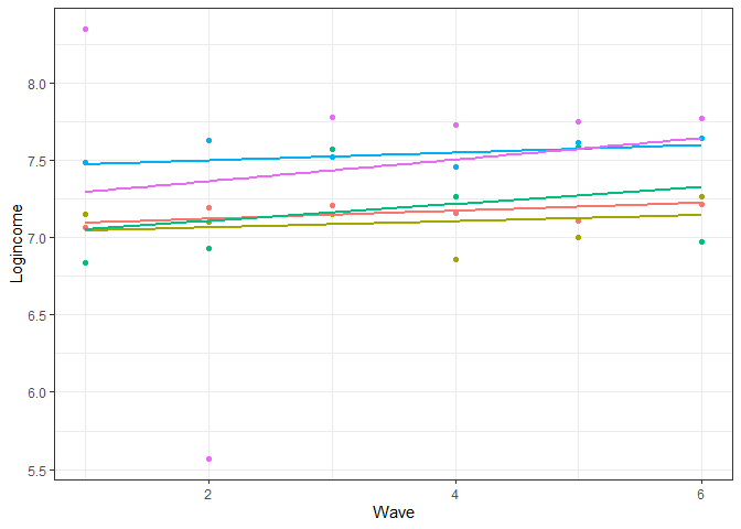
  Code
  
  usl$pred_m2 <- predict(m2) usl %>% filter(pidp %in% 1:5) %>% # select just two individuals ggplot(aes(wave, pred_m2, color = pidp)) + geom_point(aes(wave, logincome)) + # points for observed logincome geom_smooth(method = lm, se = FALSE) + # linear line based on prediction theme_bw() + # nice theme labs(x = "Wave", y = "Logincome") + # nice labels theme(legend.position = "none")
  
  Different slopes for each person

Example: Varying Slopes (Categorical) Varying Intercepts (link)

In the past, these types of {lme4} models had convergence issues, the article shows various atypical formulations for fitting these data. I didn’t have any problems fitting this model, but for higher dim data… who knows. There’s also code for data simulation.
- Tried a cross effects specification and it was worse — i.e. higher AIC and lower negative log likelihood.

Data
Varying Slopes and Intercepts

Variables and Packages

Code

library(tidyverse); library(lmerTest)
data(Machines, package = "nlme")

# for some reason worker is an ordered factor.
machines <- Machines |> 
  mutate(Worker = factor(Worker, 
                         levels = 1:6, 
                         ordered = FALSE)) |> 
  rename(worker = Worker, brand = Machine) |> 
  group_by(brand, worker) |> 
  mutate(avg_score = mean(score)) 

glimpse(machines)
#> Rows: 54
#> Columns: 4
#> Groups: brand, worker [18]
#> $ worker    <fct> 1, 1, 1, 2, 2, 2, 3, 3, 3, 4, 4, 4, 5, 5, 5, 6, 6, 6, 1, 1, 1, 2, 2, 2, 3, 3, 3, 4, 4, 4, 5, 5, 5, 6…
#> $ brand     <fct> A, A, A, A, A, A, A, A, A, A, A, A, A, A, A, A, A, A, B, B, B, B, B, B, B, B, B, B, B, B, B, B, B, B…
#> $ score     <dbl> 52.0, 52.8, 53.1, 51.8, 52.8, 53.1, 60.0, 60.2, 58.4, 51.1, 52.3, 50.3, 50.9, 51.8, 51.4, 46.4, 44.8…
#> $ avg_score <dbl> 52.63333, 52.63333, 52.63333, 52.56667, 52.56667, 52.56667, 59.53333, 59.53333, 59.53333, 51.23333, …

score (response) is a rating of quality of a product produced by a worker using a brand of machine.

EDA

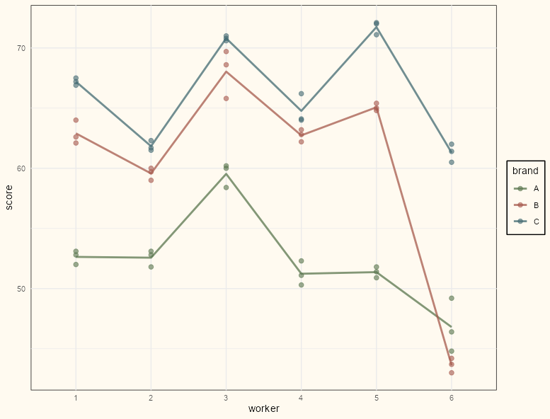
Code

ggplot(machines,
       aes(x = worker, y = score, group = brand, color = brand)) + 
  geom_point(size = 2, 
             alpha = 0.60) +
  geom_path(aes(y = avg_score), 
            size = 1, 
            alpha = .75) +
  scale_color_manual(values = notebook_colors[4:7]) +
  theme_notebook()

There does seem to be variability between workers which makes a mixed model a sensible choice.
There’s a line cross between brands B and C for worker 6 which would indicate a potential interaction in a linear model

Model

mod_brand_worker_vsvi <- 
  lmer(score ~ brand + (1 + brand | worker),
       data = machines)
summary(mod_vs_vi)

#> Linear mixed model fit by REML. t-tests use Satterthwaite's method #> ['lmerModLmerTest']
#> Formula: score ~ brand + (1 + brand | worker)
#>    Data: machines
#> 
#> REML criterion at convergence: 208.3
#> 
#> Scaled residuals: 
#>      Min       1Q   Median       3Q      Max 
#> -2.39357 -0.51377  0.02694  0.47252  2.53338 
#> 
#> Random effects:
#>  Groups   Name        Variance Std.Dev. Corr       
#>  worker   (Intercept) 16.6392  4.0791              
#>           brandB      34.5540  5.8783    0.48      
#>           brandC      13.6170  3.6901   -0.37  0.30
#>  Residual              0.9246  0.9616              
#> Number of obs: 54, groups:  worker, 6
#> 
#> Fixed effects:
#>             Estimate Std. Error     df t value Pr(>|t|)    
#> (Intercept)   52.356      1.681  5.001  31.152 6.39e-07 ***
#> brandB         7.967      2.421  4.999   3.291 0.021708 *  
#> brandC        13.917      1.540  4.999   9.036 0.000278 ***
#> ---
#> Signif. codes:  0 ‘***’ 0.001 ‘**’ 0.01 ‘*’ 0.05 ‘.’ 0.1 ‘ ’ 1
#> 
#> Correlation of Fixed Effects:
#>        (Intr) brandB
#> brandB  0.463       
#> brandC -0.374  0.301

Fixed Effects
- (Intercept) = 52.36 is the grand mean score for brand A
- brandB = 7.97 says switching from brand A to brand B increases the grand mean score by 7.97 points on average.
  - Similar for the brandC effect
Random Effects
- (Intercept) = 52.36 is the between-subject variance of each worker’s average score for brand A in relation to the grand mean score for brand A
- brandB = 7.97 and brandC = 13.92 are how much the fixed effect of brand B vs. A, and C vs. A varies per person.
- Residual = 0.96 is the within-subject standard deviation of each worker’s rating in relation to their average rating.
  - 2 standard deviations = 2 $\cdot$ 0.96 = 1.82
  - For 95% of the population of workers, their individual ratings fluctuate around the average rating by $\pm$ 1.82
- The correlation matrix in the summary is a bit difficult to decipher without the column names.
```
vcov_mats <- lme4::VarCorr(mod_vs_vi)
attributes(vcov_mats$worker)$correlation
#>             (Intercept)    brandB     brandC
#> (Intercept)   1.0000000 0.4838743 -0.3652566
#> brandB        0.4838743 1.0000000  0.2965069
#> brandC       -0.3652566 0.2965069  1.0000000
```

Example: Crossed or Nested Effects (link)
- Data, Description
  - stress is job-related stress for nurses
  - treatment is a training program to deal with stress
mod_stress_nested <- lmer( stress ~ age + sex + experience + treatment + wardtype + hospsize + (1 | hospital/ward), data = nurses ) summary(mod_stress_nested) #> REML criterion at convergence: 1640 #> #> Random effects: #> Groups Name Variance Std.Dev. #> ward:hospital (Intercept) 0.3366 0.5801 #> hospital (Intercept) 0.1194 0.3455 #> Residual 0.2174 0.4662 #> Number of obs: 1000, groups: ward:hospital, 100; hospital, 25 #> #> Fixed effects: #> Estimate Std. Error df t value Pr(>|t|) #> (Intercept) 5.379585 0.184686 46.055617 29.128 < 2e-16 *** #> age 0.022114 0.002200 904.255524 10.053 < 2e-16 *** #> sexFemale -0.453184 0.034991 906.006741 -12.952 < 2e-16 *** #> experience -0.061653 0.004475 908.841521 -13.776 < 2e-16 *** #> treatmentTraining -0.699851 0.119767 72.776723 -5.843 1.34e-07 *** #> wardtypespecial care 0.050807 0.119767 72.775457 0.424 0.67266 #> hospsizemedium 0.489400 0.201547 21.963644 2.428 0.02382 * #> hospsizelarge 0.901527 0.274824 22.015667 3.280 0.00342 ** #> ---
- As noted in Specifations and Notation >> Nested Efects, Crossed Effects, either specification in {lme4} outputs the same results with the stipulation that the nesting variable (ward) is unique.
  
  It is not unique in this case, so in order to use the crossed specification, you’d have to use wardid.
  
  *The interpretations are also the same.*
- There are no random effects correlations. This is a nested effects specification, so nested effects are being treated as crossed effects which are assumed independent.
The intercept seems to be the grand mean at the ward-level, which is the base level of this hierarchical structure. It’s not the sample grand mean exactly, but it’s close. And it’s closer than any of the other group averages I tried. Also, there are multiple measures (i.e. multiple nurses) for each ward, so it isn’t the overall mean either.
mod_stress_nested_basic <- lmer(stress ~ 1 + (1 | hospital / ward), data = nurses) fixef(mod_stress_nested_basic) #> (Intercept) #> 5.000986 avg_per_ward <- nurses |> summarize(avg_ward = mean(stress), .by = ward) # ward or wardid = same results mean(avg_per_ward$avg_ward) #> [1] 5.001627
- BTW, taking the average for each ward within each hospital, then averaging by hospital is the same as just averaging by ward (I always have to prove this to myself).
Interpretation
- ward:hospital (Intercept) = 0.3366
  
  ward:hospital is essentially just ward for intepretation purposes
  
  Between-Subject variance in the stress levels among different wards within the same hospital.
  
  A larger ward variance says there are significant differences in the average stress between different wards while in the same hospital.
  
  Ward-level factors such as workload, team dynamics, patient acuity, etc. may explain such effects
- hospital (Intercept) = 0.1194
  
  Between-Subject variance for hospitals after accounting for wards.
  
  A larger hospital variance says there are substantial differences in the average stress levels between hospitals, even after controlling for the ward effects.
  
  Hospital-level factors such as hospital policies, resources, management, etc. may explain such effects.
- Residual = 0.2174
  
  Within-Subject variance that remains after accounting for wards and hospital between-subject variance
  
  Possible sources of variability would include: skill level, levels of training, attention to detail, mood, fatigue, etc.
- Ward’s variance is 50% of the total variance so it is more important than subject-level factors or hospital-level factors in explaining stress.
Visualize Random Effects
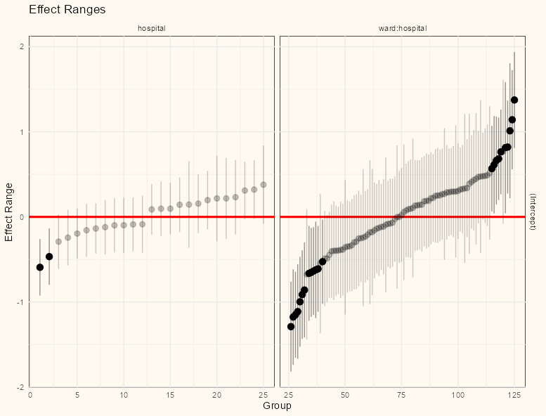
library(merTools) REsim(mod_stress_nested) |> plotREsim() + theme_notebook()
- The visual makes it apparent there’s much more variance in the random effects for ward than there is for hospital.

Example: {ggeffects} Error Bar Plot

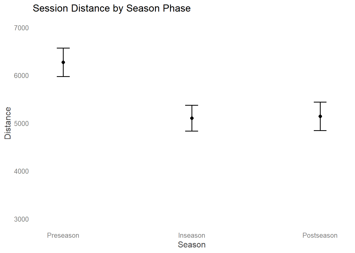
library(ggeffects); library(ggplot2)
# create plot dataframe
# Has 95% CIs for fixed effects and lists random effects
plot_data <- 
  ggpredict(
    fit, 
    terms = c("Season")
  )

#create plot
plot_data |> 
  #reorder factor levels for plotting
  mutate(
    x = ordered(
          x, 
          levels = c("Preseason", "Inseason", "Postseason")
        )
  ) |> 
  #use plot function with ggpredict objects
  plot() +
  #add ggplot2 as needed
  theme_blank() + 
  ylim(c(3000,7000)) + 
  ggtitle("Session Distance by Season Phase")

Description:
- Outcome: Distance
- Fixed Effect: Season
- Random Effect: Athlete

Example: {tidymodels} Varying Intercepts

lmer_spec <- 
  linear_reg() %>% 
  set_engine("lmer")

tidy_mod <- 
  lmer_spec %>% 
  fit(pp60 ~ position + toi + (1 | player),
      data = df)

tidy_mod
## parsnip model object
## 
## Linear mixed model fit by REML ['lmerMod']
## Formula: pp60 ~ position + toi + (1 | player)
##    Data: data
## REML criterion at convergence: 115.8825
## Random effects:
##  Groups  Name        Std.Dev.
##  player  (Intercept) 0.6423 
##  Residual            0.3452 
## Number of obs: 80, groups:  player, 20
## Fixed Effects:
## (Intercept)    positionF          toi 
##    -0.16546      1.48931      0.06254

BMLR Chapter 8: Multilevel Models

Beyond Multiple Linear Regression, Chapter 8: Introduction to Multilevel Models
Variable Types
- Level One: variables measured at the most frequently occurring observational unit
  - i.e. Variables that (for the most part) have different values for each row
  - i.e. Vary for each repeated measure of a subject and vary between subjects
- Level Two: variables measured on larger observational units
  - i.e. Constant for each repeated measure of a subject but vary between each subject
Data Description in the Examples
- na (outcome) - Negative Affect (i.e. Performance Anxiety)
- large - binary
  - large = 1 means the performance type is a Large Ensemble
  - large = 0 means the performance type is either a Solo or Small Ensemble
- orch - binary
  - orch = 1 means the instrument is Orchestral
  - orch = 0 means the instrument is either a Keyboard or it’s Vocal
Two-Stage Model
- The 2-stage model shows a clearer depiction of how a multi-level model is fit in principle
  - 2-stage model uses Ordinary Least Squares to fit a system of regression equations in stages
  - The multi-level model fits a composite of that system of equations using Maximum Likelihood Estimation
- Process
  - Level 1 models are fitted for each subject/unit
  - Using the estimated level 1 intercepts and slopes as outcome variables, Level 2 intercept and slope models respectively are fit
  - The errors from the Level 2 models are the random effects
- Issues
  - Weights every subject the same regardless of the number of repeated observations
  - Responds to missing individual slopes (i.e. subjects never exposed to treatment) by simply dropping those subjects
  - Does not share strength effectively across subjects
- Specification
  - Level 1
    
    \[ Y_{ij} = a_i + b_i \text{large}_{ij} + \epsilon_{ij} \]
    - $b_i$ is the fixed effect for subject/unit $i$ and observation $j$ (i.e. each subject has repeated observations)
  - Level 2
    
    \[ \begin{align} a_i &= \alpha_0 + \alpha_1 \text{orch}_i + u_i \\ b_i &= \beta_0 + \beta_1 \text{orch}_i + v_i \end{align} \]
    - $u_i$ and $v_i$ are the random effects for subject/unit $i$
    - $a_i$ is the true (i.e. not estimated since no hat) mean of performance anxiety (outcome) when subject plays solos or small ensembles (large = 0)
    - $b_i$ is the true mean difference in performance anxiety (outcome) for subject_i between large ensembles and other performance types (large contrast)

Multi-Level

Process
- Level 1 and Level 2 equations have been combined through substitution then reduced into a composite model
- Parameters estimated through Maximum Likelihood Estimation
Misc
- Error Distribution
  - Correlation between parameters is accounted for using a multivariate normal distribution estimated through a variance-covariance matrix of the error terms (aka random effects) of each Level (see link for details)
- Adding Level 1 variables to a model formula should change within-person variability ($\hat\sigma^2$ and $\hat\sigma$)
  - Even without adding a Level 1 variable, small changes could occur due to numerical estimation procedures used in likelihood-based parameter estimates
- Optimization methods
  - Usually very little difference between ML and REML parameter estimates
  - Restricted Maximum Likelihood (REML) is preferable when the number of parameters is large or the primary interest is obtaining estimates of model parameters, either fixed effects or variance components associated with random effects
  - Maximum Likelihood (MLE) should be used if nested fixed effects models are being compared using a likelihood ratio test, although REML is fine for nested models of random effects that have the same fixed effects.
- P-Values
  - Can’t be calculated because the exact distribution of the test statistics under the null hypothesis (no fixed effect) is unknown, primarily because the exact degrees of freedom is not known
  - Rule of Thumb: t-values (ratios of parameter estimates to estimated standard errors) with absolute value above 2 indicate significant evidence that a particular model parameter is different than 0
  - Packages that do report p-values of fixed effects typically using conservative assumptions, large-sample results, or approximate degrees of freedom for a t-distribution
    - Using {lmerTest} will produce a summary of {lme4} with pvals for coefficients
  - Parametric Bootstrap can be used to approximate the distribution of the likelihood test statistic and produce more accurate p-values by simulating data under the null hypothesis
- Model Comparison
  - Pseudo-R²
    - See below in Simple to Complex Model Building Workflow >>
      - Random Slopes and Intercepts Model (with 1 covariate)
      - Random Slopes and Intercepts Model (with 2 covariates)
  - AIC, BIC
    - See Random Intercepts (with 2 covariates)
  - Likelihood Ratio Test (LR-Test)
    - See Random Slopes and Intercepts Model (with 3 covariates)
Composite Specification

\[ Y_{ij} = [\alpha_0 + \alpha_1 \text{orch}_i + \beta_0 \text{large}_{ij} + \beta_1 \text{orch}_i \text{large}_{ij}] + [u_i + v_i \text{large}_{ij} + \epsilon_{ij}] \]
- Composite model of level 1 and level 2 equations
- Random Slopes and Intercepts Model (with 2 covariates)
- Fixed Effects: $\alpha_0$, $\alpha_1$, $\beta_0$ and $\beta_1$
- $u_i + v_i \cdot \text{large}_{ij} + \epsilon_{ij}$ is the interesting part.
  - This part has all the error terms and any variables in the Level 2 equations
  - The first part is a typical regression with interaction terms.
Interpretation
- See Two-stage model for definitions for $a_i$ and $b_i$
  - Keyboardists and Vocalists (orch_i = 0)
    
    \[ \begin{align} a_i &= \alpha_0 + u_i \\ b_i &= \beta_0 + v_i \end{align} \]
  - Orchestral Instrumentalists (orch_i = 1)
    
    \[ \begin{align} a_i = (\alpha_0 + \alpha_1) + u_i \\ b_i = (\beta_0 + \beta_1) + v_i \end{align} \]
- Mean Performance Anxiety (outcome) when:
  - Keyboardists or Vocalists (orch = 0) play solos or small ensembles (large = 0): $\alpha_0$
  - Keyboardists or vocalists (orch = 0) play large ensembles (large = 1): $\alpha_0 + \beta_0$
  - Orchestral instrumentalists (orch = 1) play solos or small ensembles (large = 0): $\alpha_0 + \alpha_1\alpha_0 + \alpha_1$
  - Orchestral instrumentalists (orch = 1) play large ensembles (large = 1): $\alpha_0 + \alpha_1 + \beta_0 + \beta_1$
Model Summary (using lmer4::lmer())
```
#>     Linear mixed model fit by REML ['lmerMod'] 
#> A)  Formula: na ~ orch + large + orch:large + (large | id) 
#>         Data: music 
#> B)  REML criterion at convergence: 2987 

#> B2)      AIC      BIC  logLik deviance df.resid 
#>         3007    3041    -1496    2991      489 

#>     Random effects: 
#>       Groups  Name        Variance Std.Dev. Corr 
#> C)  id      (Intercept)    5.655   2.378         
#> D)            large        0.452   0.672   -0.63 
#> E)  Residual              21.807   4.670         
#> F)  Number of obs: 497, groups:  id, 37 

#>     Fixed effects: 
#>                 Estimate Std. Error t value 
#> G)  (Intercept)  15.930      0.641  24.83 
#> H)  orch          1.693      0.945   1.79 
#> I)  large        -0.911      0.845  -1.08 
#> J)  orch:large   -1.424      1.099  -1.30
```
- Definitions
  - A: How our multilevel model is written in R, based on the composite model formulation.
  - B: Measures of model performance. Since this model was fit using REML, this line only contains the REML criterion.
  - B2: If the model is fit with ML instead of REML, the measures of performance will contain AIC, BIC, deviance, and the log-likelihood.
  - C: Estimated variance components ($\hat \sigma^2_u$ and $\hat \sigma_u$) associated with the intercept equation in Level Two. (between-unit variability)
  - D: Estimated variance components ($\hat \sigma^2_v$ and $\hat \sigma_v$) associated with the large ensemble (large = 1) effect equation in Level Two. (Also between-unit variability but just for the slope)
    - Also, in the “Corr” column, the estimated correlation ($\hat \rho_{uv}$) between the two Level Two error terms.
  - E: Estimated variance components ($\hat \sigma^2$ and $\hat \sigma$ associated with the Level One equation. (within-unit variability)
  - F: Total number of performances where data was collected (Level One observations = 497) and total number of subjects (Level Two observations = 37).
  - G: Estimated fixed effect ($\hat \alpha_0$) for the intercept term, along with its standard error and t-value (which is the ratio of the estimated coefficient to its standard error).
  - H: Estimated fixed effect ($\hat \alpha_1$) for the orchestral instrument (orch = 1) effect, along with its standard error and t-value.
  - I: Estimated fixed effect ($\hat \beta_0$) for the large ensemble (large = 1) effect, along with its standard error and t-value.
  - J: Estimated fixed effect ($\hat \beta_1$) for the interaction between orchestral instruments (orch = 1) and large ensembles (large = 1), along with its standard error and t-value.
- Interpretations
  - Fixed effects:
    - $\hat \alpha_0 = 15.9$ — The estimated mean performance anxiety (outcome) for solos and small ensembles (large = 0) for keyboard players and vocalists (orch = 0) is 15.9.
    - $\hat \alpha_1 = 1.7$ — Orchestral instrumentalists (orch = 1) have an estimated mean performance anxiety (outcome) for solos and small ensembles (large = 0) which is 1.7 points higher than keyboard players and vocalists (orch = 0).
    - $\hat \beta_0 = −0.9$ — Keyboard players and vocalists (orch = 0) have an estimated mean decrease in performance anxiety (outcome) of 0.9 points when playing in large ensembles (large = 1) instead of solos or small ensembles (large = 0).
    - $\hat \beta_1 = −1.4$ — Orchestral instrumentalists (orch = 1) have an estimated mean decrease in performance anxiety (outcome) of 2.3 points when playing in large ensembles (large = 1) instead of solos or small ensembles (large = 0), 1.4 points greater than the mean decrease among keyboard players and vocalists (orch = 0).
      - He’s calculating simple slope/marginal effect (See Regression, Interactions) and choosing to use that as the interpretation for the interaction term
        
        From Ch. 1 (link): “We interpret the coefficient for the interaction term by comparing slopes under fast and non-fast conditions; this produces a much more understandable interpretation for a reader than attempting to interpret the -0.011 (interaction coef) directly”
        
        Fast and non-fast are levels of a main effect and a term in the interaction.
      - Calculation: The interaction is the difference in slopes for one interaction variable (e.g. large) at different values of the other interaction variable (e.g. orch)
        
        Regression eq (ignoring the random effects part):
        
        $\hat Y_i = 15.93 + 1.693\text{orch}_i - 0.911\text{large} − 1.424\text{orch}_i \times \text{large}_i$
        
        Examining the large slope so only dealing with terms that contain “large”
        
        large = 1 is reference category in the interaction that the coefficient is associated with so it remains constant
        
        When orch = 0 and large = 1, the slope for large is -0.911 = $\hat \beta_0$
        
        $- 0.911\text{large} − 1.424\text{orch}_i \times \text{large}_i = -0.911 \times 1 - 1.424 \times \boldsymbol{0} \times 1 = -0.911 = \hat \beta_0$
        
        When orch = 1 and large = 1, the slope for large is -2.335 (uses this one for his interpretation)
        
        $- 0.911\text{large} − 1.424\text{orch}_i \times \text{large}_i = -0.911 \times 1 - 1.424 \times \boldsymbol{1} \times 1 = -0.911 - 1.424 = -2.335$ (i.e. “decrease… of 2.3 points”)
        
        The difference in these slopes is the interaction coefficient: $-2.335 - (-0.911) = -1.424$
  - Variance components
    - $\hat \sigma_u = 2.4$ — The estimated standard deviation of performance anxiety (outcome) for solos and small ensembles (large = 0) is 2.4 points, after controlling for instrument (orch) played.
    - $\hat \sigma_v = 0.7$ — The estimated standard deviation of differences in performance anxiety (outcome) between large ensembles (large = 1) and other performance types (large = 0) is 0.7 points, after controlling for instrument (orch) played.
    - $\hat \rho_{uv} = −0.64$ — The estimated correlation between performance anxiety scores (outcome) for solos and small ensembles (large = 0) and increases in performance anxiety (outcome) for large ensembles (large = 1) is -0.64, after controlling for instrument (orch) played.
      - Those subjects with higher performance anxiety scores for solos and small ensembles tend to have greater decreases in performance anxiety for large ensemble performances.
    - $\hat \sigma = 4.7$ — The estimated standard deviation in residuals for the individual regression models is 4.7 points.

Model Building Workflow: Simple to Complex

Workflow should include:
- Fixed effects that allow one to address primary research questions
- Fixed effects that control for important covariates at all levels
- Investigation of potential interactions
- Variables that are centered where interpretations can be enhanced
- Important variance components
- Removal of unnecessary terms
- A final model that tells a “persuasive story parsimoniously”
Model Comparison (Also see multi-level >> misc >> p-values & model comparison)
- LR-Test for nested models
- AIC, BIC for unnested models
- Consider models that involve removing terms that have t-stats < |2|
Models
- Unconditional Means (aka Random Intercepts)
- Random Slopes and Intercepts Model (with 1 covariate)
- Random Slopes and Intercepts Model (with 2 covariates)
- Random Intercepts (with 2 covariates)
- Random Slopes and Intercepts Model (with 3 covariates)
- Final Model

Unconditional Means (aka Random Intercepts)

Specification
- Level 1: $Y_{ij} = a_i + \epsilon_{ij} \quad \text{where}\: \epsilon \sim \mathcal{N}(0, \sigma^2)$
  - $a_i$ is the true mean response of all observations for subject_i
- Level 2: $a_i = \alpha_0 + u_i \quad \text{where} \: u_i \sim \mathcal{N}(0, \sigma^2_u)$
  - Each subject’s intercept is assumed to be a random value from a normal distribution centered at $\alpha_0$ with variance $\sigma^2_u$.
- Composite: $Y_{ij} = \alpha_0 + u_i + \epsilon_{ij}$

Model

#Model A (Unconditional means model)
model.a <- lmer(na ~ 1 + (1 | id), REML = T, data = music)
##  Groups  Name        Variance Std.Dev.
##  id      (Intercept)  4.95    2.22   
##  Residual            22.46    4.74
##  Number of Level Two groups =  37
##            Estimate Std. Error t value
## (Intercept)    16.24    0.4279  37.94

Interpretation
- $\hat \alpha_0 = 16.2$ — The estimated mean performance anxiety score across all performances and all subjects.
- $\hat \sigma^2 = 22.5$ — The estimated variance in within-person deviations.
- $\hat \sigma^2_u = 5.0$ (rounded from 4.95) — The estimated variance in between-person deviations.
- ICC
  
  \[ \hat \rho = \frac{\text{between-person variability}}{\text{total variability}} = \frac{\hat \sigma^2_u}{\hat \sigma^2_u + \hat \sigma ^2} = \frac{5.0}{5.0 + 22.5} = 0.182 \]
  - 18.2% of the total variability in performance anxiety scores are attributable to differences among subjects.
    - *For plain random intercepts models only*, you can also say this same number says that the average correlation for any pair of responses from the same individual is a moderately low 0.182.
  - As $\rho$ approaches 0: responses from an individual are essentially independent and accounting for the multilevel structure of the data becomes less crucial.
  - As $\rho$ approaches 1: repeated observations from the same individual essentially provide no additional information and accounting for the multilevel structure becomes very important.
  - Effective Sample Size (ESS): The number of independent pieces of information we have for modeling
    - With $\rho$ near 0: ESS approaches the total number of observations.
    - With $\rho$ near 1: ESS approaches the number of subjects in the study.

Random Slopes and Intercepts Model (with 1 covariate)

1 - Level 1
Specification
- Level 1: $Y_{ij} = a_i + b_i \text{large}_{ij} + \epsilon_{ij}$
- Level 2
  
  \[ a_i = \alpha_0 + u_i \\ b_i = \beta_0 +v_i \]
- Composite
  
  \[ \begin{aligned} &Y_{ij} = [\alpha_0 + \beta_0 \text{large}_{ij}] + [u_i + v_i \text{large}_{ij} + \epsilon_{ij}] \\ &\begin{aligned} \text{where}\quad \epsilon &\sim \mathcal{N}(0, \sigma^2) \: \text{and}\\ \left[ \begin{array}{cc} u_i \\ v_i \end{array} \right] &\sim \mathcal{N} \left(\left[\begin{array}{cc} 0\\0 \end{array}\right], \left[\begin{array}{cc} \sigma^2_u\\\rho\sigma_u \sigma_v \quad \sigma^2_v \end{array}\right]\right) \end{aligned} \end{aligned} \]

Model

model.b <- lmer(na ~ large + (large | id), data = music)
##  Groups  Name        Variance Std.Dev. Corr 
##  id      (Intercept)  6.333  2.517         
##          large        0.743  0.862    -0.76
##  Residual            21.771  4.666
##  Number of Level Two groups =  37
##            Estimate Std. Error t value
## (Intercept)  16.730    0.4908  34.09
## large        -1.676    0.5425  -3.09

Interpretation
- $\hat \alpha_0 = 16.7$ — The mean performance anxiety level (outcome) before solos and small ensemble performances (large = 0).
- $\hat \beta_0 = −1.7$ — The mean decrease in performance anxiety (outcome) before large ensemble performances (large = 1).
  - Subjects had a performance anxiety level of 16.7 before solos and small ensembles, and their anxiety levels were 1.7 points lower, on average, before large ensembles, producing an average performance anxiety level before large ensembles of 15.0
  - Statistically significant since |t-value| > 2
- $\hat \sigma^2 = 21.8$ — The variance in within-person deviations.
- $\hat \sigma^2_u = 6.3$ — The variance in between-person deviations in performance anxiety scores (outcome) before solos and small ensembles (large = 0).
- $\hat \sigma^2_v = 0.7$ — The variance in between-person deviations in increases (or decreases) (slope) in performance anxiety scores (outcome) before large ensembles (large = 1).
- $\hat \rho_{uv} = −0.76$ (Corr column)
  - Slopes and intercepts are negatively correlated
  - A strong negative relationship between a subject’s performance anxiety (outcome) before solos and small ensembles (large = 0) (Intercept) and their (typical) decrease in performance anxiety (Slope) before large ensembles (large = 1) .
Pseudo-R² (Not always a reliable performance measure)
- Unconditional Means vs Random Intercepts and Slopes
  
  \[ \text{Psuedo R}^2_{L1} = \frac{\hat \sigma^2 (\text{Model A}) - \hat\sigma^2(\text{Model B})}{\hat \sigma^2(\text{Model A})} = \frac{22.5 - 21.8}{22.5} = 0.031 \]
  - Where Model A: Unconditional Means; Model B: Random intercepts and slopes
  - FYI
    - $\text{percent decrease} = \frac{\text{original value} - \text{new value}}{\text{orginal value}}$
      - pseudo-R² uses this one
      - If negative, it’s a percent increase.
    - $\text{percent increase} = \frac{\text{new value} - \text{original value}}{\text{original value}}$
      - If negative, it’s a percent decrease.
- Positive value means Model B is an improvement over Model A
  - Means the variance in Model B’s error terms is smaller than Model A’s, and therefore better fits the data. (I think)
- The estimated within-person variance $\hat \sigma^2$ decreased by 3.1% (from 22.5 to 21.8) from the unconditional means model
- Implies that only 3.1% of within-person variability in performance anxiety scores can be explained by performance type
- Values of $\hat \sigma^2_u$ and $\hat \sigma^2_v$ from Model B cannot be compared to between-person variability from Model A using pseudo-R², since the inclusion of performance type has changed the interpretation of these values
- Issues
  - “Because of the complexity of estimating fixed effects and variance components at various levels of a multilevel model, it is not unusual to encounter situations in which covariates in a Level Two equation for the intercept (for example) remain constant (while other aspects of the model change), yet the associated pseudo R-squared values differ or are negative.” (?)

Random Slopes and Intercepts Model (with 2 covariates)

1 - Level 1; 1 - Level 2
Specification, Model, Interpretation (see Multi-Level section above)
- Says the large effect (slope) varies across subjects/units
Pseudo-R²

\[ \begin{align} \text{Psuedo R}^2_{L2_u} &= \frac{\hat \sigma^2_u (\text{Model B}) - \hat\sigma^2_u(\text{Model C})}{\hat \sigma^2_u(\text{Model B})} = \frac{6.33 - 5.66}{6.33} = 0.106 \\ \text{Psuedo R}^2_{L2_v} &= \frac{\hat \sigma^2_v (\text{Model A}) - \hat\sigma^2_v(\text{Model B})}{\hat \sigma^2_v(\text{Model A})} = \frac{0.74 - 0.45}{0.74} = 0.392 \end{align} \]
- Model B is Random Slopes and Intercepts Model (with 1 covariate)
- Model C is Random Slopes and Intercepts Model (with 2 covariates)
- The addition of Level 2 variable, orch, in Model C:
  - (Top) Decreased the between-person variability in mean (intercept) performance anxiety (outcome) before solos and small ensembles (large = 0) by 10.6%
  - (Bottom) Decreased the between-person variability in the effect (slope) of large ensembles (large = 1) on performance anxiety (outcome) by 39.2%

Random Intercepts (with 2 covariates)

1 - Level 1; 1 - Level 2
Instead of assuming that the large ensemble (large) effects, after accounting for instrument played (orch), vary by individual, we are assuming that large ensemble effect is fixed across subjects.
Specification
- Level 1: $Y_{ij} = a_i + b_i \text{large}_{ij} + \epsilon_{ij}$
- Level 2
  
  \[ \begin{align} &a_i = \alpha_0 + \alpha_1 \text{orch}_i + u_i\\ &b_i = \beta_0 + \beta_1 \text{orch}_i \\ &\text{where}\: \epsilon \sim \mathcal{N}(0, \sigma^2)\: \text{and} \: u_i \sim \mathcal{N}(0, \sigma^2_u) \end{align} \]
  - Only difference is the random effect/error term, $v_i$, isn’t specified
- Composite
  - Not given, but probably very similar to the previous model just without $v_i$

Model

model.c2 <- lmer(na ~ orch + large + orch:large + (1|id), data = music)
##  Groups  Name        Variance Std.Dev.
##  id      (Intercept)  5.13    2.27   
##  Residual            21.88    4.68
##  Number of Level Two groups =  37
##            Estimate Std. Error t value
## (Intercept)  15.9026    0.6187  25.703
## orch          1.7100    0.9131   1.873
## large        -0.8918    0.8415  -1.060
## orch:large   -1.4650    1.0880  -1.347

Interpretation
- Same as previous model except there’s no between-units variation estimate for the slope (see previous model and multi-level model section)
- Estimates are similar to the previous model’s. Largest difference seems to be the between-unit variation for the Intercept (5.66 vs 5.13)
Comparison
```
        df  AIC
model.c  8 3003
model.c2 6 2999
        df  BIC
model.c  8 3037
model.c2 6 3025
```
- Model C is the previous model and Model C2 is this model
- Both criterion pick this model to predict best
- The more complex model (e.g. varying intercepts and varying slopes) doesn’t always perform best

Random Slopes and Intercepts Model (with 3 covariates)

1 - Level 1; 2 - Level 2
MPQnem has been centered (mean = 31.63)
- Otherwise some interpretations would involve MPQnem = 0 when the minimum score is 11 which would make the interpretation nonsensical
Specification
- Level 1: $Y_{ij} = a_i + b_i \text{large}_{ij} + \epsilon_{ij}$
- Level 2
  
  \[ \begin{align} a_i = \alpha_0 + \alpha_1 \text{orch}_i + \alpha_2 \text{MPQnem}_i + u_i \\ b_i = \beta_0 + \beta_1 \text{orch}_i + \beta_2 \text{MPQnem}_i + v_i \end{align} \]
- Composite
  
  \[ Y_{ij} = [\alpha_0 + \alpha_1 \text{orch}_i + \alpha_2 \text{mpqnem}_i + \beta_0 \text{large}_{ij} + \beta_1 \text{orch}_i \text{large}_{ij} + \beta_2 \text{mpqnem}_i \text{large}_{ij}] + [u_i + v_i \text{large}_{ij} + \epsilon_{ij}] \]

Model

model.d <- lmer(na ~ orch + mpqnem + large +
                    orch:large + mpqnem:large +
                    (large | id),
                    data = music)
##  Groups  Name        Variance Std.Dev. Corr 
##  id      (Intercept)  3.286  1.813         
##          large        0.557  0.746    -0.38
##  Residual            21.811  4.670
##  Number of Level Two groups =  37
##               Estimate Std. Error t value
## (Intercept)   16.25679    0.54756 29.6893
## orch           1.00069    0.81713  1.2246
## cmpqnem        0.14823    0.03808  3.8925
## large         -1.23484    0.84320 -1.4645
## orch:large    -0.94927    1.10620 -0.8581
## cmpqnem:large -0.03018    0.05246 -0.5753

Interpretation
- Compared to Random Slopes and Intercepts Model (with 2 covariates):
  - Directions of the effects of instrument (orch) and performance type (large) are consistent
  - Effect sizes and levels of significance are reduced because of the relative importance of the negative emotionality (mpqnem) term
- $\alpha_0 = 16.26$ — The estimated mean performance anxiety (outcome) for solos and small ensembles (large = 0) is 16.26 for keyboard players and vocalists (orch=0) with an average level of negative emotionality at baseline (mpqnem = 31.63)
- $\hat \alpha_1 = 1.00$ — Orchestral instrument (orch = 1) players have an estimated mean performance anxiety (outcome) level before solos and small ensembles (large = 0) which is 1.00 point higher than keyboardists and vocalists (orch = 0), controlling for the effects of baseline negative emotionality.
- $\hat \sigma^2 = 0.15$ — A one point increase in baseline negative emotionality (mpqnem = 0) is associated with an estimated 0.15 mean increase in performance anxiety (outcome) levels before solos and small ensembles (large = 0), after controlling for instrument (orch).
- $\hat \beta_0 = −1.23$ — Keyboard players and vocalists (orch = 0) with an average level of baseline negative emotionality levels (mpqnem = 31.63) have an estimated mean decrease in performance anxiety level (outcome) of 1.23 points before large ensemble performances (large = 1) compared to other performance types (large = 0).
  - See multi-level>> interpretation for explainer on the interaction slope interpretations
- $\hat \beta_1 = −0.95$ — After accounting for baseline negative emotionality (mpqnem = 0), orchestral instrument players (orch = 1) have an estimated mean performance anxiety level (outcome) before solos and small ensembles (large = 0) which is 1.00 point higher than keyboardists and vocalists (orch = 0), while the mean performance anxiety (outcome) of orchestral players (orch = 1) is only .05 points higher before large ensembles (large = 1) (a difference of .95 points).
  - See multi-level >> interpretation for explainer on the interaction slope interpretations
- $\hat \beta_2 = −0.03$ — After accounting for instrument, a one-point increase in baseline negative emotionality is associated with an estimated 0.15 mean increase in performance anxiety levels before solos and small ensembles, but only an estimated 0.12 increase before large ensembles (a difference of .03 points).
LR-Test for comparing nested models
```
drop_in_dev <- anova(model.d, model.c, test = "Chisq")
#>         npar  AIC  BIC logLik  dev Chisq Df      pval
#> model.c    8 3007 3041  -1496 2991    NA NA        NA
#> model.d   10 2996 3039  -1488 2976 14.73  2 0.0006319
```
- MLE must be used instead of REML to estimate the parameters of each model
- model.d is the current and more complex model, Random Slopes and Intercepts Model (with 3 covariates)
- model.c is the less complex model, Random Slopes and Intercepts Model (with 2 covariates)
- Process
  - The likelihood is larger (and the log-likelihood is less negative) under the larger model (Model D);
  - $\text{Chisq} = 14.734 = -2 \cdot (-1488 - (-1496))$
  - Using dof = 2, signifying the number of additional terms in Model D, we obtain a p-value of .0006.
- A p-value < 0.05 indicates the difference in log-likelihoods is significantly different from 0, and therefore the more complex model, model.d, fits the data better.
- Note: dropping the mpqnem:large term which has a t-stat < |2| (-0.5753) produces a better model than model.d according the LR-test

Final Model

Description
- One of other valid final models
- Performance type categorical is no longer collapsed into the binary “large” ensemble/not large and is has now been collapsed into the binary, solo, not solo
- Audience categorical has been transformed to dummies: students, juried, public with instructor as the reference category.
- Varying/random slopes for previous, students, juried, public, and solo
- mpqnem is in the solo level 2 equation, so the combined model has an interaction between the two in the fixed effects.
Specification
- Level 1: $Y_{ij} = a_i + b_i \text{previous}_{ij} + c_i \text{students}_{ij} + d_i \text{juried}_{ij} + e_i \text{public}_{ij} + f_i \text{solo}_{ij} + \epsilon_{ij}$
- Level 2
  
  \[ \begin{align} a_i &= \alpha_0 + \alpha_1 \text{mpqpem}_i + \alpha_2 \text{mpqab}_i + \alpha_3 \text{orch}_i + \alpha_4 \text{mpqnem}_i + u_i \\ b_i &= \beta_0 + v_i \\ c_i &= \gamma_0 + w_i \\ d_i &= \delta_0 + x_i \\ e_i &= \epsilon_0 + y_i \\ f_i &= \zeta_0 + \zeta_1 \text{mpqnem}_i + z_i \end{align} \]
  - Variance-Covariance matrix
    
    \[ \left[\begin{array}{cc} u_i\\v_i\\w_i\\x_i\\y_i\\z_i \end{array} \right] \sim \mathcal{N} \left( \left[\begin{array}{cc} 0\\0\\0\\0\\0\\0\end{array} \right], \begin{bmatrix} \sigma_u^2 \\ \sigma_{uv} & \sigma_v^2 \\ \sigma_{uw} & \sigma_{vw} & \sigma^2_w \\ \sigma_{ux} & \sigma_{vx} & \sigma_{wx} & \sigma_x^2 \\ \sigma_{uy} & \sigma_{vy} & \sigma_{wy} & \sigma_{xy} & \sigma_{y}^2 \\ \sigma_{uz} & \sigma_{vz} & \sigma_{wz} & \sigma_{xz} & \sigma_{yz} & \sigma_z^2 \end{bmatrix} \right) \]
  - 6 variance terms and 15 correlation terms at Level Two, along with 1 variance term at Level One.
    - The number of correlation terms is equal to the number of unique pairs among Level Two random effects

Model

# Model F (One - of many - reasonable final models)
model.f <- lmer(na ~ previous + students + juried + 
    public + solo + mpqpem + mpqab + orch + mpqnem + 
    mpqnem:solo + (previous + students + juried + 
    public + solo | id), REML = T, data = music)

##  Groups  Name        Variance Std.Dev. Corr       
##  id      (Intercept) 14.4802  3.805               
##          previous     0.0707  0.266    -0.65     
##          students     8.2151  2.866    -0.63  0.00
##          juried      18.3177  4.280    -0.64 -0.12
##          public      12.8094  3.579    -0.83  0.33
##          solo         0.7665  0.876    -0.67  0.47
##  Residual            15.2844  3.910     
##             
##  0.84           
##  0.66  0.58     
##  0.49  0.21  0.90
## 
##  Number of Level Two groups =  37
##            Estimate Std. Error t value
## (Intercept)  8.36883    1.91369  4.3731
## previous    -0.14303    0.06247 -2.2895
## students     3.61115    0.76796  4.7022
## juried       4.07332    1.03130  3.9497
## public       3.06453    0.89274  3.4327
## solo         0.51647    1.39635  0.3699
## mpqpem      -0.08312    0.02408 -3.4524
## mpqab        0.20377    0.04740  4.2986
## orch         1.53138    0.58384  2.6230
## mpqnem       0.11465    0.03591  3.1930
## solo:mpqnem  0.08296    0.04158  1.9951

Interpretation
- In general
  - Performance anxiety (outcome) is higher when a musician is performing in front of students, a jury, or the general public rather than their instructor
    - students, juried, and public are indicator variables created from the audience categorical variable (so that “Instructor” is the reference level in this model)
  - Performance anxiety (outcome) is lower for each additional diary the musician previously filled out
    - previous is the number of previous diary entries filled out by that individual
  - Musicians with lower levels of positive emotionality (mpqpem) and higher levels of absorption (mpqab) tend to experience greater performance anxiety (outcome)
  - Those who play orchestral instruments experience (orch = 1) more performance anxiety than those who play keyboards or sing (orch = 0)
- Key terms
  - $\hat \alpha_4 = 0.11$ (mpqnem, fixed) — A one-point increase in baseline level of negative emotionality (mpqnem) is associated with an estimated 0.11 mean increase in performance anxiety (outcome) for musicians performing in an ensemble group (solo=0), after controlling for previous diary entries (previous), audience (dummy vars), positive emotionality (mpqpem), absorption (mpqab), and instrument (orch).
  - $\hat \zeta_1 = 0.08$ (solo:mpqnem, fixed) — When musicians play solos (solo = 1), a one-point increase in baseline level of negative emotionality (mpqnem) is associated with an estimated 0.19 mean increase in performance anxiety (outcome), 0.08 points (73%) higher than musicians playing in ensemble groups (solo = 0), controlling for the effects of previous diary entries (previous), audience (dummy vars), positive emotionality (mpqpem), absorption (mpqab), and instrument (orch).
    - See multi-level >> interpretation for explainer on the interaction slope interpretations
- Addressing the researchers’ primary hypothesis:
  - After controlling for all these factors, we have significant evidence that musicians with higher levels of negative emotionality (mpqpem) experience higher levels of performance anxiety (outcome), and that this association is even more pronounced (interaction) when musicians are performing solos (solo = 1) rather than as part of an ensemble group (solo = 0).

BMLR Chapter 9: Longitudinal Data

Beyond Multiple Linear Regression, Chapter 9: Two-Level Longitudinal Data
Research Questions
- Which factors most influence a school’s performance in Minnesota Comprehensive Assessment (MCA) testing?
- How do the average math MCA-II scores for 6th graders enrolled in charter schools differ from scores for students who attend non-charter public schools? Do these differences persist after accounting for differences in student populations?
- Are there differences in yearly improvement between charter and non-charter public schools?
Data Answers
- Within school—changes over time
- Between schools—effects of school-specific covariates (charter or non-charter, urban or rural, percent free and reduced lunch, percent special education, and percent non-white) on 2008 math scores and rate of change between 2008 and 2010.
Misc
- Missing data is a common phenomenon in longitudinal studies