Investing
Misc
Resources
- Tidy Finance - R and Python versions
- Tidy Portfolio Management in R
- Machine Learning for Factor Investing
- Advances in Financial Machine Learning - de Prado (R >> Documents >> Financial)
- Machine Learning for Algorithmic Trading
- Github repo with the code that’s referred to in the book
Packages
- CRAN Task View
- {tidyquant}
- Download and clean data - Daily stock prices (historical), key statistics (real-time), key ratios (historical), financial statements, dividends, splits, economic data from the FRED, FOREX rates from Oanda
- Performance Analysis and Portfolio Analysis
- {IBrokers} - R API to Interactive Brokers Trader Workstation
- Interactive Brokers is an international brokerage firm specializing in electronic execution in products ranging from equities to bonds, options to futures, as well as FX, all from a single account
- {rPublic} - The Public Trading API allows clients to access their brokerage accounts, request market data, and place stock/etf/option orders.
- {TTR} - A collection of over 50 technical indicators for creating technical trading rules. The package also provides fast implementations of common rolling-window functions, and several volatility calculations.
- {zipline-reloaded} - Backtesting and live-trading engine by crowd-sourced investment fund Quantopian
- {pyfolio} - Performance and risk analysis for financial portfolios
- {skfolio} - Portfolio optimization built on top of scikit-learn. It offers a unified interface and tools compatible with scikit-learn to build, fine-tune, and cross-validate portfolio models.
- {alphalens} - Performance analysis of predictive stock factors
- {PyBroker} - A backtesting engine; A framework is designed for developing algorithmic trading strategies, with a focus on strategies that use machine learning. Easily create and fine-tune trading rules, build powerful models, and gain valuable insights into your strategy’s performance.
- {empyrical} - Common financial risk and performance metrics. Used by zipline and pyfolio.
- {riskfolio-lib} - Tools for quantitative strategic asset allocation or portfolio optimization
Tools
For portfolio construction in general, positions are optimized using Expected Returns, Return Variance (i.e. volatility), and Co-Movements (i.e. covariance) in order to maximize Risk Adjusted Returns.
Technical vs Fundamental Analysis
- Technical analysis in many cases tends to amplify stock price trends because many technical traders buy when stocks are rising and sell when they fall.
- Fundamental analysis on the contrary often shows mean-reverting behaviour because its adherents try to buy undervalued stocks and sell overvalued ones
Smoothers
- Simple Moving Average (SMA) is simple, easy to implement but reacts slowly to recent price changes due to equal weighting of all prices in the window.
- Exponential Moving Average (EMA) reacts faster to recent price changes due to more weight to the latest prices.
- Kalman Filter is more sophisticated and can adaptively weigh incoming measurements based on their estimated noise level, potentially providing superior results in many applications. However, it has key parameters that must be tuned to get good results.
Strategies
- Notes from
- Hedgefund - factor rotations (longer term)
- Something about futures - factor tilts (shorter term)
- Harvesting Risk Premia
- Should be the primary focus of independent traders.
- General Process
- Intentionally expose your portfolio to diverse sources of risk that tend to be rewarded (noting that not all risks are rewarded)
- Manage risk sensibly so no risk dominates at any time
- Be patient and chill (the hardest part for most)
- Examples: 60/40 stock/bond portfolio
- Economically-sensible, statistically-quantifiable slow-converging inefficiencies
- These are noisy tendencies for assets to trade too cheap or expensive at certain times due to behavioral or structural effects. Slow to converge and must be analyzed in aggregated datasets. Generally, these edges are less reliable than risk premia harvesting.
- After mastering Harvesting Risk Premia, add a little of this over time.
- Requirements
- To understand why the inefficiency would persist.
- Faster converging metrics around what we’re exploiting so we’re not the last to know when the inefficiency disappears.
- Patience and discipline to keep swinging the bat – you have to let the noisy edge play out over a large number of bets.
- Examples: Momentum effects, seasonal regularities, effects due to indexing inclusion/exclusion, probably style factors (momentum, value, carry, quality, low vol), and most medium frequency statistical arbitrage approaches.
- Resources
- Expected Returns by Antti Ilmanen
- Efficiently Inefficient by Lasse Pedersen
- Positional Option Trading by Euan Sinclair (which literally gives you stuff to trade)
- Active Portfolio Managementby Grinhold and Kahn
- Fast-converging supply-demand imbalances
- Short term supply and demand imbalances create dislocations in prices which fast traders can “disperse” by trading against them and offsetting risk elsewhere. It carries risks because we can’t trade instantaneously.
- Require significant investment in infrastructure and staff, so isn’t practical for “home gamers.”
- Examples
- Arbitrage: Buy futures on Shanghai INE and buy a similar contract cheaper on Singapore SGX for a profit (after costs).
- Trend-Equities Strategy
- See Bonds versus CTAs for Diversification
- Allocates 100% to the S&P 500 if the 12-month return is positive measured every month, otherwise 100% is allocated to short-term U.S. Treasury bills
- This strategy in a 60-40 proportion along with CTAs performs well in low-yielding market environments.
Misleading chart (Thread)
- No transaction costs
- No fees
- No taxes
- US “exceptionalism”
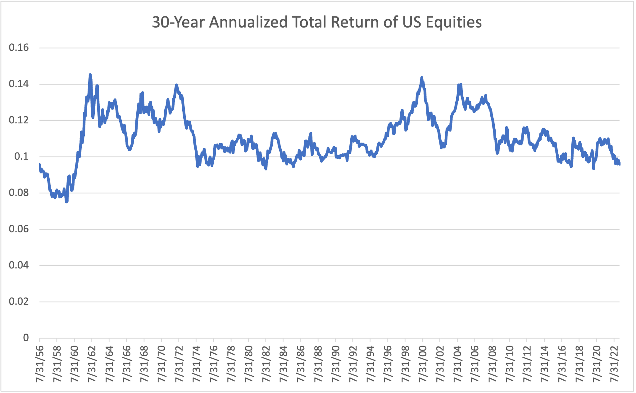
- Overlapping time period analysis
- Example: if I look at 1920-1950 and then 1921-1951, twenty eight of the thirty data points are overlapping. So there’s not a lot of “unique” data in this set.
- Nominal vs real returns - Time weighted vs dollar weighted returns
Workflow
From Machine Learning for Algorithmic Trading 
Any market forecasting model, especially involving short term horizons, should probably have a random walk in an ensemble. (Is the Market Just Random Noise?)
The Invesco QQQ ETF
- Tracks the Nasdaq-100 Index, which includes 100 of the largest non-financial companies listed on the Nasdaq stock exchange
- Heavily weighted towards technology companies
- Often used as a benchmark for the performance of the technology sector and growth stocks in general
- A popular underlying asset for options trading, adding to its significance in derivatives markets
Walk-Forward Optimisation: This method involves optimizing the strategy on a rolling basis, where a portion of the data is used to optimize parameters, and the next portion is used to test the strategy. The process is repeated across the entire dataset.
Considerations
- Costs that need to be accounted for when backtesting
- Transaction costs
- Fees
- Slippage
- Taxes
- A model that performs well in a specific market condition may incur substantial losses when the market shifts, be it due to news, events, or economic changes.
- See Finance, Snippets >> Misc >> Test Assumptions
- Beware of survivorship bias when backtesting algorithms
- Example: S&P 500
- A trader is creating an algorithm to predict prices of all the stocks in the S&P 500. If the trader uses the current roster of companies, the list only includes companies that have made it to now without shutting down or losing so much value they drop off the list. The trader should use the list of companies as it was at the start of the training data.
- Example: S&P 500
- Answer the questions: ‘does my model make money when it is supposed to?’ as well as ‘Does my model lose money when it is supposed to?’.
- Validating that it loses money when it’s supposed to is approach that helps to confirm the profits weren’t being generated by noise.
- Monte Carlo Simulations can help. Valid for some models more than others, this involves running the strategy through a large number of simulated market scenarios, with different sequences of returns, to assess how it performs under various market conditions.
- Parameter Sensitivity Analysis: If your model works with a 200 period moving average and dies with a 210 period moving average, you’re doomed. But see how far you can take this analysis. You can drive research by testing a myriad of permutations to confirm a hypothesis, rather than ‘spit out a model’. This doesn’t just go for indicators – what about stress testing commissions or slippage?
- Take other measures into consideration besides overall performance metrics such as Sharpe Ratio or Calmar Ratio
- How many trades does your strategy generate?
- What are the trade level statistics?
- Ask yourself what it would take for your assumption to break down. How could you prepare for that?
- Simpler models are easier to diagnose if concerns come up.
- Use proper stop-loss and position sizing strategies to manage risk
- Iteratively using the same data to design and modify a strategy can lead to overfitting, where the strategy becomes overly tailored to the data and performs poorly in real-world trading.
- Ignorance of macro-economic indicators and trends can result in unexpected market moves, significantly impacting algorithmic strategies and their performance.\
- There are 435 choices for start and end dates of each monthly investment cycle
- i.e. Easy to have a selective endpoints fallacy for an investment strategy.
60/40 Portfolio Strategy
- Misc
- {QSTrader}
- Notes from - The 60/40 Benchmark Portfolio
- Description
- 60/40 US Equities/Bonds strategy is a simple long-term investment approach that is widely utilised in the investment industry. It seeks to ensure that at any point during the lifetime of the investment that 60% of account equity is invested in one or more assets representing a broad selection of US equities (such as an S&P500 ETF), while 40% of account equity is invested in one or more assets representing a broad selection of US treasury bonds (such as a treasury bond ETF).
- Since the actual percentage allocations of each asset class can deviate over time due to relative growth of the respective assets a ‘rebalance’ approach is often carried out. This means that trades are issued on a relatively infrequent basis to buy/sell amounts of each asset class to periodically bring the account equity allocations back into the 60/40 split. For the particular strategy implemented here we are using an end of month rebalance frequency.
- More balanced implementations include Bridgewater’s All-Weather portfolio and Risk Parity strategies generally, which attempt to equalize risk across assets or sources of risk premia.
Factor-based
- Misc
- Todo: beta, size, and value factors
- Resources
- Criteria for an factor To be considered for using in investments (Swedroe and Berkin)
- Must have provided a premium that was persistent across long periods and different economic regimes
- Pervasive across countries, regions, sectors, and even asset classes
- Robust to various definitions
- Investable (it held up after implementation costs)
- Intuitive (there are logical risk-based or behavioral-based explanations for the premium, providing the rationale that it should continue to exist).
- Acceleration is typically defined as the quarter-on-quarter change to a particular factor.
- Quality
- Characteristics: low earnings volatility, low financial leverage, high gross profitability, high return on equity, low operating leverage, high asset turnover, low accruals (high earnings quality), low equity dilution, and low idiosyncratic stock risk.
- Misc
- Quality, Factor Momentum, and the Cross-Section of Returns - Overview of a paper on quality acceleration that uses profitability, growth, payout, and safety to measure Quality. It gives the proxy measures for each characteristic.
- Packages
- {qmj} - Produces quality scores for each of the US companies from the Russell 3000, following the approach described in “Quality Minus Junk”
- Indexes:
- MSCI
Index - Select “Quality” from the Index Suite dropdown and either the Regional or Country tab. It gives return percentages for various year intervals.
See R >> Documents >> Finance >> Reference >> MSCI_Quality_Indexes_Methodology_May2022 for further details on their methodology.
Calculates their quality score for each security by averaging Z-Scores of three winsorized fundamental variables: Return on Equity, Debt to Equity and Earnings Variability.
After averaging the z-scores \(Z_{\text{avg}}\), the Quality Score is determined by:
\[ \text{QS} = \left\{ \begin{array}{lcl} 1 + Z, & Z \gt 0 \\ (1-Z)^{-1}, & Z \lt 0 \end{array}\right. \]
Fundamental Variables:
Return on Equity (ROE) - Shows how effectively a company uses investments to generate earnings growth
\[ \mbox{ROE} = \frac{\text{Trailing 12-Month Earnings per Share}}{\text{Latest Book Value per Share}} \]
Debt to Equity (D/E) - Measures a company’s leverage
\[ \mbox{D/E} = \frac{\text{Total Debt}}{\text{Book Value}} \]
Earnings Variability: The standard deviation of y-o-y earnings per share growth over the last five fiscal years. Measures how smooth earnings growth has been.
- S&P
- Indices categorized by market cap size
- Based on Return on Equity, Accruals Ratio, and Financial Leverage Ratio
- See R >> Documents >> Finance >> Reference >> methodology-sp-quality-indices for details on methodology
- MSCI
- Momentum
- Cross-Sectional (aka Relative) - Stocks are ranked according to momentum and the top ranked stocks are bought. The bottom ranked stocks may be shorted.
- Time-Series (aka Absolute or Trend)- Past performance of a single stock is evaluated and it’s determined whether its trend will continue.
- Factor - It applies the concept of momentum towards factors.
- e.g. If the value factor (investing in undervalued stocks) has performed well in recent periods, a factor momentum strategy would increase exposure to the value factor. Conversely, if the momentum factor (investing in past winners) has underperformed, the strategy might reduce exposure to the momentum factor.
Momentum Strategies
- Misc
Notes from
- Minimizing the Risk of Cross-Sectional Momentum Crashes
- See article for more details and links to resources
- Cross-Sectional Momementum - Investing in previous winners and short-selling previous losers
- Minimizing the Risk of Cross-Sectional Momentum Crashes
Types of Momentum: Cross-Sectional (aka Long-Short) and Absolute (aka Trend, Time Series)
Individual investors can utilize momentum strategies without incurring additional costs by incorporating momentum into trading decisions. For example, when rebalancing, they can delay purchases of assets with negative momentum and delay sales of assets with positive momentum.
Momentum Portfolios with higher trend clarity (measured by R2) have higher returns than portfolios with lower trend clarity. Trend clarity is a driver of momentum. (article)
High Trend Clarity 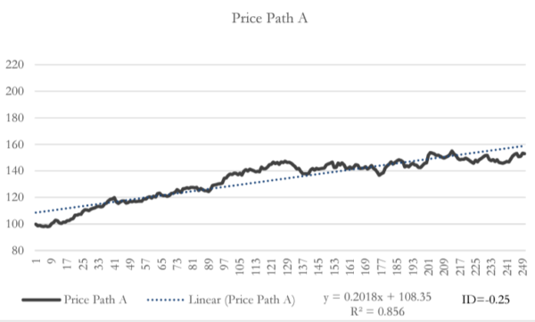
Low Trend Clarity 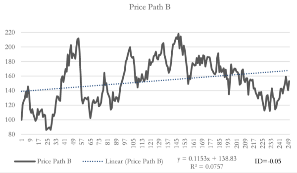
- The impact of trend clarity on momentum was more pronounced in smaller stocks, where information diffusion tends to be slower.
- A more pronounced effect of trend clarity on momentum occurs during periods of high sentiment.
- the clarity of the price trend closely aligned with earnings surprises (Standardized Unexpected Earnings (SUE)). As SUE changes and the steepness of changes in SUE increased, so did trend clarity, suggesting that positive or negative news instigated the clear price trend. As the magnitude of SUE diminished and the trend reversed, indicating a deficiency of fundamentals to back the extrapolation by trend followers.
Momentum Tactical Asset Allocation Strategy
- Misc
- Description
- The US sector momentum strategy is a long-only dynamic tactical asset allocation strategy that attempts to exceed the performance of simply going long the S&P500.
- At the end of every month the strategy calculates the holding period return (HPR) based momentum of all of the SPDR sector ETFs (the ticker symbols of which begin with the prefix XL) and selects the top N to invest in for the forthcoming month, where N is usually between 3 and 6.
- In the implementation given here the HPR momentum is calculated over the previous 126 days (approximately six months of business days) and the top three sector ETFs are chosen for the portfolio.
- The portfolio allocation is equally weighted between each of these three sector ETFs. Irrespective of changes in signal the portfolio is rebalanced once per month to weight the assets equally.
- Risk
- Momentum displays a huge tail risk, as there are short but persistent periods of highly negative return which occur in reversals from bear markets, when the momentum portfolio displays a negative market beta and momentum volatility is high.
- Investors have experienced huge drawdowns—momentum exhibits both high kurtosis and negative skewness.
- Momentum volatility increases in times of momentum crashes
- “…strong relationship between the level of high-yield spreads and the one-month returns to the momentum factor. Specifically, tight high-yield spreads are associated with robust momentum premia, while elevated spreads (400-700 basis points) predict weaker returns. The right signal to move out of the momentum strategy—or even to initiate strong bets on reversals—has historically been when spreads exceed 700 basis points.”
- The “high-yield spread is not a particularly useful predictor of the forward returns of the ‘winner’ portfolio,” however, the high-yield spread “significantly predicts momentum crashes by identifying when the ‘loser’ portfolios will experience positive reversals.”
- Downturns are forecastable — occurring following market declines and when market volatility is high (contemporaneous with market rebounds) — but also that there are systematic strategies that have been shown to historically reduce crash risk. Smoler-Schatz showed that the high-yield spread is one of them.
Dual Momentum Sector Rotation
- Notes from Simulation of Gary Antonacci’s Dual Momentum Sector Rotation Strategy
- Characteristics
- Conditions for investing offensively or defensively: the 12-month momentum of the S&P500 (absolute mom)
- List of offensive investment vehicles: the 11 sectors that make up the S&P500 index (relative strength)
- Number of sectors to be selected when the strategy is invested offensively: 4
- Sector selection criteria: 12-month momentum
- List of defensive investment vehicles: US Aggregate Global Bond or Money Market (Cash)
- Number of instruments to be selected when the strategy is invested defensively: 1
- Process
- 12-month momentum of the S&P500 used to decide whether the market is in an uptrend or a downtrend, i.e. to invest offensively or defensively.
- If the S&P500 is in an uptrend, invest offensively. In this case, the allocation is spread evenly over the 4 sectors with the highest 12-month momentum, 25% each.
- If fewer than 4 sectors have positive momentum, then the remainder not invested offensively is allocated to a defensive position.
- If the S&P500 is trending downwards (negative momentum), I invest defensively. In this case, I allocate the entire portfolio to US government bonds or the money market, depending on which market has offered the highest returns over the last 12 months.
- Those familiar with the GEM strategy will note that the author initially recommended using only US government bonds as a defensive asset. However, since interest rates have fallen so much over the last 10 years, since the publication of his study, it now seems more reasonable to compare the US government bond market with the performance of the money market, in order to select the market that offers the best risk/return trade-off.
- Calculate 12-month momentum: ( Price at the end of the month – Price 12 months ago ) / ( Price 12 months ago )
- Momentum calculations and any arbitrages are carried out at the end of each month.
- Comparison
- Cumulative Performance: DMSR vs. SPY vs. GEM
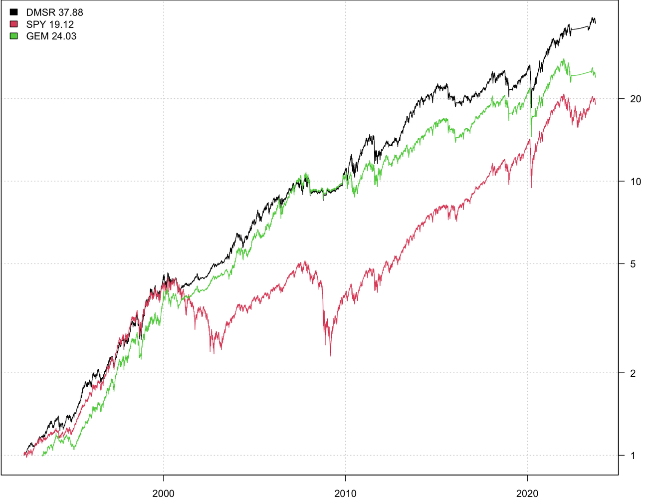
- Simple Cumulative Performance (%) is computed every month (I think)
- Rate of Return
\[ \text{RoR} = \frac{\text{Ending Value} - \text{Starting Value}}{\text{Starting Value}} \times 100 \] - Cumulative Performance (CP)
\[ \text{CP} = (1 + \text{RoR}_1) \times (1 + \text{RoR}_2) \times \cdots \times (1 + \text{RoR}_n) - 1 \]
- Rate of Return
- Simple Cumulative Performance (%) is computed every month (I think)
- Statistics
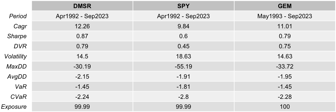
- Cumulative Performance: DMSR vs. SPY vs. GEM
Momentum-based Long & Short
- tl;dr: Over the past 23yrs, the Average Annual Return (%) was between 18% and 27% depending on the various parameters you decide on, but the maximum drawdowns are very large — between 56% and 80%. It was hit hard during recessions, so the strategy needs adjusted.
- Notes from: Momentum-based Long & Short Equities Portfolio
- General Strategy:
- Every month (or week, or 15 days), we will rank a universe of stocks by a momentum factor;
- Then, we will long the top decile and short the bottom decile;
- At the beginning of every month, we will re-balance.
- Parameters Tested:
- Stock Universe Sizes: top 150, 500, and 1,000 stocks in terms of market cap;
- Rebalancing Frequencies: weekly, biweekly, and monthly.
- Process
- On the first day of every month, we rank the top 150 stocks in terms of market cap according to their momentum factor;
- We long the top 15 and short the bottom 15, with equal weights to each stock;
- We use all the available capital (the cash available and the proceeds from the shorts) to long the stocks.
- Results
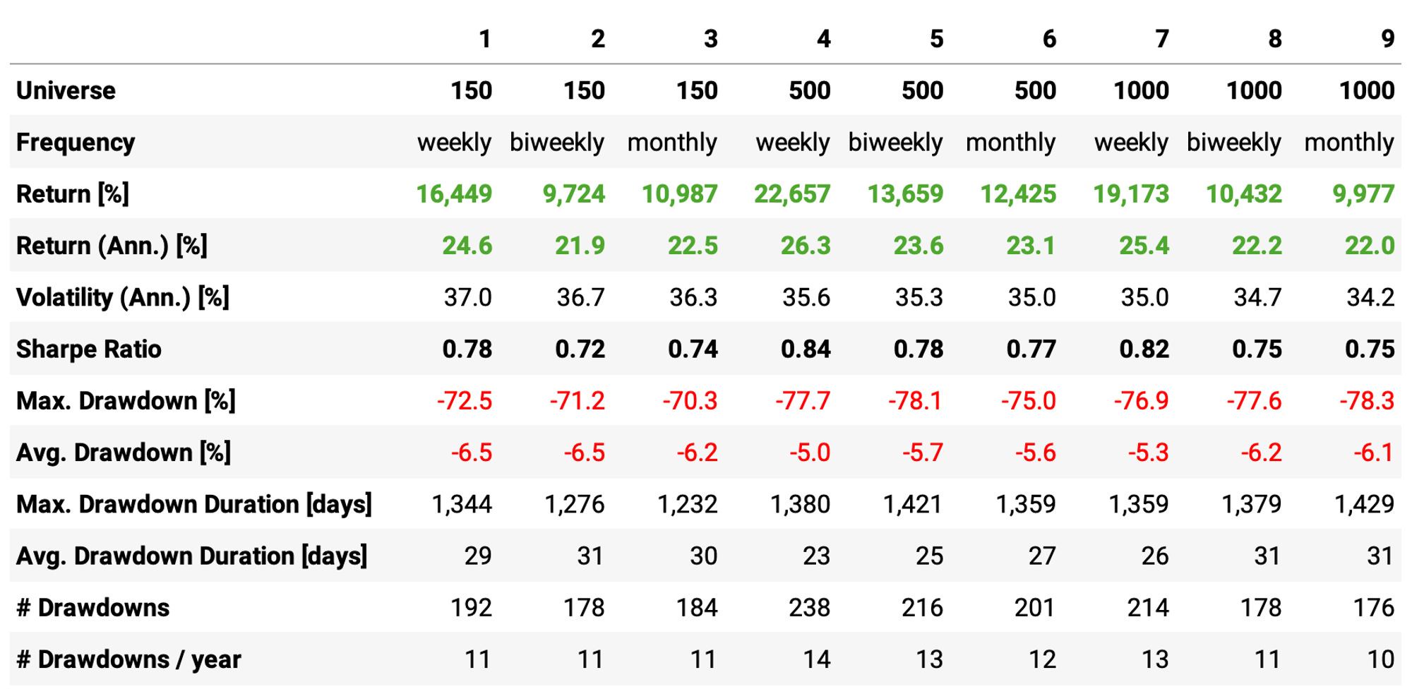
- Best Results: experiment 4 with a universe of 500 stocks and weekly rebalancing
- Market Regime Filter applied to reduce maximum drawdown
- Process
- If, on a rebalancing date, the S&P 500 is below its 200-day moving average, then move to 100% cash;
- Resume trading when the S&P 500 comes back above to the 200-SMA
- Results:
- Achieved a 0.91 Sharpe, the highest in all experiments;
- The maximum drawdown reduced to 57%, same as benchmark, and unfortunately still too high;
- Invested 80% of the time, so the exposure-adjusted return would be 23.4%.
- Process
- Other risk reducing strategies
- Tried but failed:
- Position sizing had poor performance.
- Stop-loss orders would not only cut losers but also cut winners
- Try individual stocks and trade instruments in parallel as opportunities appear
- Try different asset classes (ETFs, futures, crypto, etc)
- Try a cross-sectional momentum strategy;
- Try a machine learning model to predict the probability of a stock to outperform (or underperform) in the near future, training this model with momentum-based signals.
- Combine with other strategies like Mean Reversion
- Tried but failed:
Volatility Targeting Portfolio
- Misc
- Volatility targeting seeks to counter the fluctuations in volatility:
- It leads to leveraging a portfolio at times of low volatility, and scaling down exposures at times of high volatility.
- This approach targets a constant level of volatility, rather than a constant notional exposure.
- Volatility clustering is a key feature of financial asset returns:
- High volatility over the recent past tends to be followed by high volatility in the near future.
- Impact on Sharpe ratio
- Volatility targeting improves the Sharpe ratio of “risk assets” (equities and credit), and that of “balanced” and “risk parity” portfolios that have a substantial allocation to these risk assets.
- For equity and credit, volatility targeting effectively introduces some momentum overlay due to the so-called leverage effect: the negative relationship between returns and changes in volatility.
- In contrast, for bonds, currencies, and commodities the impact on the Sharpe ratio is negligible.
- Impact on likelihood of tail events
- Volatility targeting reduces the likelihood of extreme returns for all asset classes.
- Importantly, “left-tail” events tend to be less severe, as they typically occur at times of elevated volatility, when a target-volatility portfolio has a scaled-down notional exposure.
Pairs Trading
- Papers
- Pairs Trading Using a Novel Graphical Matching Approach
- Application of graph theory to the selection of stock pairs. Results in robust risk-adjusted performance but also achieves annualized returns comparable to the S&P 500 with a superior Sharpe ratio
- Selection based solely upon the significance of cointegration between pairs can result in portfolios overly concentrated in a limited number of stocks, which elevates portfolio variance and diminishes risk-adjusted returns
- Utilizes of graph theory to the selection of stock pairs to decrease variance with the t-statistic from a cointegration statistical test as the weight for the edges.
- Application of graph theory to the selection of stock pairs. Results in robust risk-adjusted performance but also achieves annualized returns comparable to the S&P 500 with a superior Sharpe ratio
- Pairs Trading Using a Novel Graphical Matching Approach
- Match two trading vehicles that are highly correlated, trading one long and the other short when the pair’s price ratio diverges “x” number of standard deviations - “x” is optimized using historical data. If the pair reverts to its mean trend, a profit is made on one or both of the positions.
- Chart the relative performance (price ratio)
- The center white line represents the mean price ratio over the past two years. The yellow and red lines represent one and two standard deviations from the mean ratio, respectively.
- The potential for profit can be identified when the price ratio hits its first or second deviation. When these profitable divergences occur it is time to take a long position in the underperformer and a short position in the overachiever. (i.e. shorting the stock that’s rising in relation to the other, and buying the other stock that hasn’t risen yet)
- The revenue from the short sale can help cover the cost of the long position, making the pairs trade inexpensive to put on.
- Position size of the pair should be matched by dollar value rather than number of shares; this way a 5% move in one equals a 5% move in the other.
- As with all investments, there is a risk that the trades could move into the red, so it is important to determine optimized stop-loss points before implementing the pairs trade.
- Chart the spreads between returns
- Look for stocks that move closely together and their:
- Spreads zig-zag around zero
- Prices separately (marginally) are normally distributed and joint-normally distributed (assumes linear correlation)
- If both, then they move up AND down together (symmetric)
- If only marginally, then they probably only move in one direction together (asymmetric)
- If your two assets returns (differenced prices are stationary) do not correlate within a [0.7..0.8] correlation coefficient range at least 70% of the times (70% of all observations) then you’re probably dealing with a very bad hedging instrument
- Look to cover the remaining data points and research why correlations broke down during those periods. If you can derive a mathematical relationship you could possibly formulate an approach in which you make adjustments to the hedge ratio through an adjustment in your beta/correlation coefficient.
- Figure out the optimal time interval to retrain model due to data drift
- Rolling 20-day correlation is a common way to monitor stock correlation
- Beware of two correlated stocks that have similar Beta or some other confounding variable
- Graphical LASSO can help remove effects such as market Beta and recover real, direct relationships between stocks.
- It makes intuitive sense that in a large universe, most stocks would be conditionally independent, and Graphical LASSO is able to refine this sparsity condition by tuning it’s only parameter
- See Association, General >> Partial Correlation for a stock example
- Graphical LASSO can help remove effects such as market Beta and recover real, direct relationships between stocks.
- Copulas
- See Association, Copulas
- Measures non-linear association
- For Value-at-Risk (VAR) calculations, Gaussian copula is overly optimistic and Gumbel is too pessimistic
- Copulas with upper tail dependence: Gumbel, Joe, N13, N14, Student-t.
- Copulas with lower tail dependence: Clayton, N14 (weaker than upper tail), Student-t.
- Copulas with no tail dependence: Gaussian, Frank.
- Cointegration allows us to construct a stationary time series from two asset price series, if only we can find the magic weight, or more formally, the cointegration coefficient β. Then we can apply a mean-reversion strategy to trade both assets at the same time weighted by β. There is no guarantee that such β always exists, and you should look for other asset pairs if no such β can be found.
- See Forecasting, Statistical >> Terms
- Cointegrated assets share common nonstationary components, which may include trend, seasonal, and stochastic parts
- Might have low correlation, and highly correlated series might not be cointegrated at all.
- Describes a long-term relationship between the prices (correlation describes a short-term relationship between the returns). The resulting stationary series is the spread between the prices of both assets
- Should have similar risk exposure so that their prices move together
- Good candidates for cointegrated pairs could be:
- Stocks that belong to the same sector.
- WTI crude oil and Brent crude oil.
- AUD/USD and NZD/USD.
- Yield curves and futures calendar spreads
Mean Reversion
- IBS + High/Low Strategy
- Notes from A Mean Reversion Strategy with 2.11 Sharpe
- The logic behind this trading strategy is that the market tends to bounce back once it drops too low from its recent highs.
- Process
- Compute the rolling mean of High minus Low over the last 25 days;
- Compute the IBS indicator: (Close - Low) / (High - Low);
- Compute a lower band as the rolling High over the last 10 days minus 2.5 x the rolling mean of High minus Low (first bullet);
- Go long whenever SPY closes under the lower band (3rd bullet), and IBS is lower than 0.3;
- Close the trade whenever the SPY closing price is higher than yesterday’s high.
- Experiment: 1999–2024 QQQ ETF
- Results
Bonds
- Misc
- Packages
- {yieldcurves} - Yield Curve Fitting, Analysis, and Decomposition
- Resources
- NerdWallet Compound Interest Calculator
- Example: if you put $5,000 in a (5yr) bond with a 4% yield, assuming you reinvest your interest payments, you will have $6083 by the time it matures.
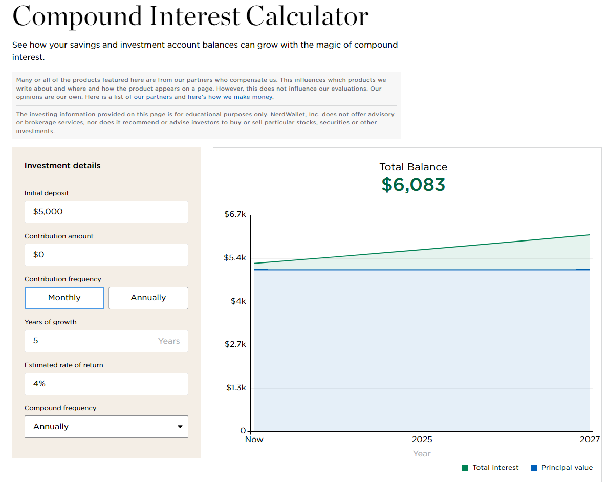
- Example: if you put $5,000 in a (5yr) bond with a 4% yield, assuming you reinvest your interest payments, you will have $6083 by the time it matures.
- Commody Trend Advisors (CTAs) are alternatives to bonds. Bonds and stocks were correlated in the 2020s while CTAs were not correlated with either.
- The SG Trend Index tracks the daily rate of return for a pool of CTAs
- Traders try to identify assets where the recent volatility has been low and have the potential to make outsized moves during so-called “tail events” – low probability occurrences that can drive big swings in asset prices.
- See Bonds versus CTAs for Diversification
- NerdWallet Compound Interest Calculator
- Notes from
- The price of a bond moves in the opposite direction to interest rates.
- As rates rise, the value of older bonds with lower coupons declines.
- Most often, people will compare the 2-year Treasury with the 10-year. So, any generic mention of the spread, in a bond context, refers to the difference in yield between these two bonds.
- Bond traders buy existing bonds in the secondary bond market, and sell them at a discount to their face value.
- The amount of the discount depends partially on how many payments are still due before the bond reaches maturity.
- The price also is a bet on the direction of interest rates. If a trader thinks interest rates on new bond issues will be lower, the existing bonds may be worth a little more.
- Zero-Coupon Bonds (aka Discount Bonds)
- Owners receive no payments for their money until the bond has matured.
- They buy the bond for an amount that is less than its face value. When it reaches its maturity, they are paid the full face value of the bond.
- Most zero-coupon bonds have a pre-set face value and therefore pay a pre-set amount of money at maturity.
- Some bonds are inflation-indexed, meaning the face value is determined at maturity. The amount paid will be based on a standard measure such as the consumer price index plus a premium.
- Considered short-term investments that typically have a maturity of no more than one year. These short-term bonds are usually called bills.
- Packages
- Questions
- Should you buy the highest-yielding bonds, or is it better to lock in good rates for longer?
- Is it better to buy bonds directly from the government, a brokerage or as part of a bond fund?
- How much do I make on bonds after taxes and fees?
- How many bonds should I buy?
- Short-Term Bonds (e.g. 2-year Treasury)
- Pros:
- Higher yields (i.e. return) than long term bonds (e.g. 10-year Treasury)
- Cons:
- When interest rates are high, you lose the opportunity (i.e. by not buying longer term bonds) to lock in a potentially higher return for longer should rates drop in the future.
- Pros:
- Bond Ladder
- Divide your investments among bonds with progressively later maturity dates.
- Investors should also choose bonds based on savings goals and how soon they will need the money
- This takes advantage of both higher short term coupons and longer term yields.
- Divide your investments among bonds with progressively later maturity dates.
- Considerations
- Check a bond’s credit ratings before you buy. A poor rating means the bond issuer, such as a corporation, is less likely to pay you back.
- This can be enticing because the issuer will likely offer you a higher interest rate. It also means they are more likely to default, which would mean you lose money.
- Watch out for hidden expenses like markup fees for purchasing an individual bond
- Can be anywhere from 1% to 5%, depending on the broker.
- You are often not buying directly from the issuer. Instead, you are buying from another investor and the price of that bond probably has shifted since it was initially issued.
- One advantage of using a brokerage is that their sites will take the guesswork out of how much the change in the market price of your bond will affect your final return.
- Taxes
- CD interest, which may at time near bond yields, is taxed as ordinary income, as high as 37%.
- The interest on Treasurys is exempt from state taxes.
- Municipal bonds are exempt from both state and local taxes if an investor buys the bond from the same state they live in.
- Corporate bonds have no tax benefits, so investors still need to pay both state and federal taxes on them.
- Bonds within a tax-sheltered account like a 401(k) or an IRA aren’t taxed until you withdraw the money
- If a zero-coupon bond is issued by a U.S. local or state government entity, interest is free from federal tax and generally exempt from state and local tax as well.
- Zero-Coupon bonds subject to taxation in the U.S. can be held in a tax-deferred retirement account, allowing their investors to avoid tax on future income.
- Check a bond’s credit ratings before you buy. A poor rating means the bond issuer, such as a corporation, is less likely to pay you back.
- Purchasing
- Treasurys and most other bonds through a brokerage such as Charles Schwab, Fidelity or Vanguard.
- Government bonds can also be bought directly from TreasuryDirect, a government website.
- Bond funds and ETFs allow you to diversify your investment.
- Bonds funds often don’t hold bonds until maturity.